Investigation on Trend Removal in Time Domain Analysis of Electrochemical Noise Data Using Polynomial Fitting and Moving Average Removal Methods
Article information
Abstract
Electrochemical noise signals in many cases exhibit a DC drift that should be removed prior to further data analysis. Polynomial fitting and moving average removal method have been used to remove trends of electrochemical noise (EN) in time domain. The corrosion inhibition of synthesized schiff base N,N′-bis(3,5-dihydroxyacetophenone)-2,2-dimethylpropandiimine on API-5L-X70 steel in hydrochloric acid solutions were used to study the effects of drifts removal methods on noise resistance calculation. Also, electrochemical impedance spectroscopy (EIS) was used to study the corrosion inhibition property of the inhibitor. The results showed that for the calculation of Rn, both methods were effective in trend removal and the polynomial with m=4 and MAR with p=40 were in agreement.
1. Introduction
Common electrochemical tools, in particular electrochemical impedance spectroscopy (EIS) and DC polarization, have been widely utilized in order to investigating the inhibition performance of various inhibitors for a long period of time. In the recent decade, an increasing interest toward applying new brand techniques such as electrochemical noise method (EN) have been spotted among corrosion researchers [1-3]. The electrochemical noise data is regarded as the natural random current and potential fluctuations around some mean value which occur on the electrode surface in the solution [4].
To understand electrochemical noise, a theoretical analysis of a completely random and brief pulse of charge generating a current and potential change is required. This indicates that the dissolution process can be treated as a series of events and the occurrence of each event is completely independent of any other event and an electrochemical reaction may be regarded as a Poisson process [5].
One of the characteristics of many natural processes is that these are both nonstationary and nonlinear. The reasons for this behavior may be different and elusive: for example, the signal may be stationary, but it may contain frequency components lower than f0 = 1/T, or there may be some slow alteration of the system under study that causes the drift, whether linear or not. In corrosion studies, progressive deterioration of the electrodes and consequent lack of stationarity is to be expected in many cases [5,6]. Any DC drift in the signal will create new, false frequency components. Also, this drift could affect the statistical result. Therefore, a critical step considering the analysis of an electrochemical current or potential noise signal is to effectively remove this DC drift, which can have a large effect upon the outcome of the data analysis [7].
Drift removal is a form of high pass (HP) filtering, consisting of suppressing the components of the signal below a certain frequency. There are two possible methods for achieving this: one is applying some kind of digital filtering after acquiring the time series, and the other is using an analog filter in real time [6,8]. There are many digital HP filtering techniques, including moving average removal (MAR), linear detrending method, regression, polynomial fitting and wavelet transform, etc [8]. For non-linear drifts, polynomial fitting and MAR methods could be selected.
Acid solutions are widely used in industries for lots of purposes, such as acid pickling, industrial acid cleaning, acid descaling and oil well acidizing [9-12]. Due to the general aggressive nature of acid solutions, this leads to corrosive attack. The strategies consist of either using corrosion resistant alloys or the use of steel with corrosion inhibitor [13-15]. Inhibition of organic compound inhibitors is due to the interaction between inhibitor molecules and the metal surface via adsorption. The inhibitor adsorption depends on parameters such as the surface charge and nature of the metal, the inhibitor structure, aggressive media type and the extent of aggressiveness and also on the nature of its interaction with metal surface [16-18]. Generally the organic compounds containing hetero atoms like O, N, S and P are found to work as very effective corrosion inhibitors [19-21].
The purpose of this paper is to study the effect of drift removal in analysis of electrochemical noise data using polynomial fitting and moving average removal to methods. Noise resistance was calculated for inhibition effect of synthesized Schiff base on corrosion of API-5L-X70 steel in hydrochloric acid solutions.
2. Experimental Section
2.1. Materials
The specimens used in electrochemical measurements were mechanically cut into 1 × 1 × 0.5 cm3, and inserted to polyester resin leaving only 1 cm2 of the surface area exposed to electrolyte. The electrical conductivity was provided by a copper wire. Tests were performed on a steel grade API-5L-X70. The surface of working electrode was mechanically abraded with 1000, 1200, and 2000 grades of emery paper and rinsed by distilled water before each electrochemical experiment. The tests were performed in 1 M HCl solution containing 0, 1 × 10⁻⁴, 2 × 10⁻⁴, 1 × 10⁻³, 2 × 10⁻³ M of BDAP Schiff base and its chemical structure is given in Fig. 1. The acid solutions (1 M HCl) were made from analytical grade 37% HCl using double-distilled water.

Chemical structure of inhibitor (N,N′-bis(3,5-dih acetophenone)-2,2-dimethylpropandiimine).
The BDAP Schiff base inhibitor (Fig. 1) was provided in high yield (95%) by the condensation of 3′,5′-Dihydroxyacetophenone (2 mmol) with 2,2-dimethylpropylenediamine (1 mmol) in a stirred ethanolic solution and heated to reflux for 6 h according to the described procedure [22]. The resulting precipitate was filtered off, washed with warm ethanol and diethyl ether. Identification of structure of synthesized Schiff base was performed by 1HNMR spectroscopy and elemental analysis. The concentration range of inhibitor employed was varied from 1 × 10⁻⁴ to 2 × 10⁻³ M.
2.2. Methods
The electrochemical measurements were carried out using computer controlled Ivium Stat potentiostat/galvanostat. To perform EIS measurement, a conventional three electrode cell including the prepared carbon steel specimen as working electrode, a Platinum rod as counter electrode and a saturated calomel reference electrode was used. EIS measurements were executed at open circuit potential (OCP) within the frequency domain 100 kHz to 0.01 Hz using a sine wave of 10 mV amplitude peak to peak. Fitting of experimental impedance spectroscopy data to the proposed equivalent circuit was done by means of home written least square software based on Marquardt method for the optimization of functions and Macdonald weighting for the real and imaginary parts of the impedance [23,24].
Electrochemical potential and current noise were simultaneously measured in a freely corroding system using two nominally identical working electrodes (coupled through the Zero Resistance Ammeter) of the same area and a saturated calomel reference electrode which was placed between the two working electrodes. The electrochemical noise data was gathered within a period of 1024 s at 0.2 s interval, which led to a frequency range from close to 1 mHz to 0.5 Hz determined by the expressions fmax = 1/2Δt and fmin = 1/NΔt where Δt and N were the sample interval and the total number of data recorded, respectively. Before electrochemical measurement the specimens were immersed in a test solution at open circuit potential (EOCP) for 20 min to attain a stable state. All experiments were carried out at 25°C. The volume of test solutions for each experiment was 150 mL.
2.3. Detrending methods
The trends electrochemical noise data might be defined as a change of the mean potential or current divided by time, i.e. (E2−E1)/(t2−t1) or (I2−I1)/(t2−t1) [25,26]. Polynomial fitting consists of fitting a polynomial of a given order to the time record and then subtracting the computed curve so as to keep the residuals. Electrochemical noise data after polynomial detrending with order m should be as follows [8]:

where X(t) is raw EN time record and Fm(t) is polynomial fitting function. In fact, Xm(t) is also the residual of the polynomial fitting with the order m.
MAR method which was described for first time by Tan et al. [27] has been used in some investigations. It is believed that any point in an array of observed potential (and current) records is composed of a real potential (and current) component and a DC trend. Considering a recorded time-potential series consisting of K data points, for any data point i we have:

Vi,noise is the real noise and is required for noise resistance calculation. Vi,DC is the DC trend component which has to be removed. According to the above assumption, average value of adjacent data points of Vi, can be taken as an estimation of the DC trend and thus the DC trend component of each noise data can be statistically calculated:

where p could be any integer number ranging from 1 to K. Therefore the DC trend in the noise data can be removed and the real component of noise data, Vi,noise, can be calculated as

It is important to note that the record analysis is strongly affected by p values. Equation (5) was used to calculate the appropriate p value for the MAR method, where Δt is the data sampling interval [28-30]:

Eqn (5), emerging from a wavelet analysis, is based on the fact that various electrochemical events have different lifetimes. Therefore, the measured signal could be over-filtered and misinterpreted in the case of too low p values.
3. Results and Discussion
3.1. Electrochemical Impedance Spectroscopy Measurements
The Bode plots of samples immersed in 1 M HCl solutions in the absence and presence of different concentrations of inhibitor are depicted in Fig. 2. Bode plots revealed one time constant for EIS response of all samples, indicating that the corrosion process is under charge transfer control in the absence and presence of different concentrations of BDAP [31]. The Bode diagrams have a similar shape throughout all tested concentrations, indicating that almost no change in the corrosion mechanism occurs due to the inhibitor addition [32-34]. The Bode resistance increases in the presence of inhibitor. This increase is more and more pronounced with increasing inhibitor concentration, which indicates the adsorption of inhibitor molecules on the metal surface. The equivalent circuit compatible with the impedance diagrams recorded in the presence of inhibitor is depicted in Fig. 3. This equivalent circuit is fitted to the experimental data and the circuit elements are obtained. For fitting of equivalent circuit to experimental impedance data, it is necessary to use a constant phase element, CPE, instead of double layer capacity to account for non-ideal behavior. The most widely accepted explanation for the presence of CPE (Qdl) behavior and depressed semicircles on solid electrodes is microscopic roughness, causing an inhomogeneous distribution in the solution resistance as well as in the double layer capacitance [35-37]. Constant phase element Qdl, Rs, and Rct can be corresponded to double layer capacitance, Qdl=Rn−1Cdln, solution resistance and charge transfer resistance, respectively [32].

Bode plots for steel in 1 M HCl without and with various concentration of DHAPP at 25°C: (1) 0, (2)1×10⁻⁴, (3) 2×10⁻⁴, (4) 1×10⁻³, (5) 2×10⁻³ M. Fitting of simulated diagram of Bode from equivalent circuit (—) on experimental Bode plots in different concentrations of inhibitor.

Equivalent circuits compatible with the experimental impedance data in Fig. 3 for corrosion of steel electrode at different inhibitor concentrations.
Table 1 illustrates the equivalent circuit parameters for the impedance spectra of corrosion of steel in 1 M HCl solution. The data indicate that increasing charge transfer resistance is associated with a decrease in the double layer capacitance. It has been reported that the adsorption of Schiff base inhibitor on the metal surface is characterized by a decrease in Qdl. The decrease in Qdl is caused by adsorption of inhibitor, indicating that the exposed area decreases. On the other hand, a decrease in Qdl, which can result from a decrease in local dielectric constant and/or an increase in the thickness of the electrical double layer, suggests that Schiff base inhibitor acts by adsorption at the metal/solution interface [23]. As the Qdl exponent (n) is a measure of the surface heterogeneity, values of n indicates that the steel surface becomes more and more homogeneous as the concentration of inhibitor increases as a result of its adsorption on the steel surface and corrosion inhibition. The increase in values of Rct and the decrease in values of Qdl with increasing the concentration also indicate that Schiff base acts as primary interface inhibitor and the charge transfer controls the corrosion of steel under the open circuit conditions [38].

Impedance spectroscopy data for corrosion of steel in 1 M HCl solution without and with different concentration of inhibitor.
3.2. Electrochemical noise measurements
Statistical methods are found to be particularly useful for the analysis of electrochemical noise data in the time domain [39]. This statistical analysis involves the estimation of the electrochemical noise resistance. The noise resistance (Rn) is obtained through dividing the standard deviation of potential by the standard deviation of current (σV/σI), which are calculated using the following equations [40].


where σV, σI and n represent the standard deviation of potential noise, the standard deviation of current noise and total number of measurements, respectively.
Fig. 4 depicts the current and potential time data of the samples immersed in 1 M HCl solution in the presence of different concentrations of inhibitor. As can be seen, voltage fluctuates around open circuit potential in the absence and presence of inhibitor. Fluctuation of potential is related to oxidation and reduction reaction on surface of the two same steel electrodes and also is due to the adsorption and desorption of inhibitor molecules. Current noise time series in the absence of inhibitor characterized by higher amplitude transients could be a qualitative indication of effectiveness of the inhibitor. Moreover, Current noise decreases with increasing inhibitor concentration which shows more adsorption of inhibitor on surface. However, because of the significant drift in the current time series shown in the Fig. 4, the DC trend should be removed to analyze the data statistically [41]. So a critical step considering the analysis of an electrochemical current or potential noise data is necessary to effectively remove this DC drift, which can have a large effect upon the outcome of the data analysis.

Current and potential noise data for carbon steel in 1 M HCl without and with various concentration of DHAPP at 25°C: (1) 0, (2)1×10⁻⁴, (3) 2×10⁻⁴, (4) 1×10⁻³, (5) 2×10⁻³ M.
Fig. 5 indicates the detrended EN time of current by polynomial fitting for steel by different m order. It can be observed that the detrended EN time data fluctuate around zero and their mean value is very small, and the general drifts are eliminated. Very low dependency of the shape, amplitude and the width of individual transients upon the value of m are visible. As can be observed from Fig. 5, some relatively long period fluctuations still exist in m=1 which makes the transient’s display unclear. After drift removal by m=4 and 9, the transients become clearer and the long period fluctuations decrease, which is attributed to removing the low frequency signals [42]. This kind of long period fluctuations is often considered as the low frequency drift that should be removed completely. In fact, the period of these fluctuations is already much shorter than the measurement period t and then should not be considered as the low frequency drift. Therefore, drift removal procedure perhaps just needs to eliminate the general trend in the EN time records [42].

The detrended current noise time series for steel in 1 M HCl in the presence of 0.002 M inhibitor with different m orders of polynomial fitting: (a) m=1, (b) m=4 and (c) m=9.
The effect of the order on Rn at different inhibitor concentrations is shown in Table 2. The variation of noise resistance in m>4 is very low and negligible. So using high m is not necessary and the polynomial fitting seems to be enough with moderate m. In addition, the values of m<6 would be recommended to avoid large calculated errors and large fluctuations at the beginning and the end of the data. Rn displays very irregular changes after drift removal with increasing m. These results demonstrate that one major problem in this method is choosing an appropriate order. So Rn is used to study the effect of order on analysis of the electrochemical noise time data. In this field, many efforts have been made to find a correlation between EIS and EN parameters [43]. It is obvious from Table 2 that in the case of time series without DC trend removal, despite the fact that all inhibited samples show inhibition behavior, no clear trend of noise resistance is observed. These observations confirm the need for DC trend removal before applying further noise analysis. Pre-treating time series with m=1,2 can also detect no continuous increasing trend for Rn. So, choosing low orders could lead to misinterpretation of the noise data. When m is equal to 3, 4 and 5, suitable trend correlation is observed between Rn and charge transfer resistance obtained by EIS and noise resistance increases with increasing inhibitor concentrations. From Table 2, it is clearly seen that with increasing order of the polynomial m>6 results in more trend removal and no continuous increasing trend for Rn. It is likely that this is accompanied by an increased loss of valuable data [5]. In addition, the noise resistance from m>6 is very close to m=4.

Effect of order m of polynomial method on Rn in different inhibitor concentrations.
Another method for detrending electrochemical noise data is MAR. Fig. 6 shows the detrended EN time records from current noise time series of steel in HCl solution with the selected p values. As seen, DC trend removal using lower values of p lead to formation of time series containing compact, narrow transients while higher p values generated wider transients in the time series. It is noted that taking lower p values in the DC trend removal can over-filter the transients related to the electrochemical events having longer lifetimes and one may risk leaving some characteristic transients undetected and misinterpret the ongoing mechanism [41]. To evaluate the effects of different p values on the time domain analysis of the noise data, different p values 3, 10, 16, 32, 50, 64, 128, 192, 256 and 400 were used to d-trending of each obtained time series in the presence of different concentrations of the inhibitor. The corresponding noise resistances of steel in inhibited and uninhibited HCl solutions with different p values are listed in Table 3. As can be seen, the changes of Rn after MAR removal with p=256 and 400 are similar to the change of Rn after polynomial removal. Moreover, its value is more approximate to Rn obtained after polynomial removal with m=3−5. The noise resistance obtained from pretreated time series using p < 256 show discrepancy from proper trend and could lead to misinterpretation of the noise data. In addition according to Fig. 6, the MAR parameter (p=400) is enough high and in agreement with polynomial fitting m=4. Also, the shape, amplitude and particularly the width of individual transients are similar. This indicates that both detrending methods are effective for drift removal of electrochemical noise data and are in agreement with each other.

The detrended current noise time series for steel in 1 M HCl in the presence of 0.002 M inhibitor with different p orders of moving average removal method (a) p=10, (b) p=64, (c) p=192, (d) p=400.
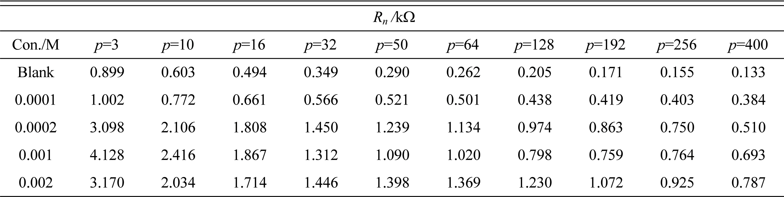
Corresponding noise resistances of the samples exposed to the inhibited and uninhibited HCl solutions, taking different p values as a MAR pretreatment.
Despite the trend correlation, it is noteworthy that the magnitude of Rn obtained by both detrending methods is different from the corresponding resistance obtained from EIS. The major reason for this is the difference between experimental conditions of techniques used to evaluate corrosion resistance of steel in acid solution. Unlike EIS, there is no need to apply external perturbation in EN measurements. In fact, data can be obtained from the natural fluctuations of current and potential at free corrosion potential. This results in the minimal interference with the system leading to a more accurate data evaluation than other electrochemical techniques. Rn is an appropriate parameter representing useful information on the inhibition effects of the inhibitors. The Rn significantly increases in the presence of the inhibitor. It is clear from the Table 3 that the noise resistance of carbon steel electrode in 1 M HCl solution significantly increases with increasing inhibitor concentrations.
The increase in Rn can be directly related to the decrease of σI because of inhibitor film formation. These results again show that the electrochemical noise measurement is a very useful method to monitor the corrosion of metals and the polynomial detrending and MAR are suitable trend removal methods.
4. Conclusion
The electrochemical noise data was analyzed in time domain for corrosion inhibition effect of synthesized Schiff base on API-5L-X65 steel in 1 M HCl solution. The following conclusions were drawn:
1. The EN method was highly sensitive to the data pretreatment, especially for the applied DC trend removal approach.
2. Polynomial fitting and moving average removal were suitable methods for detrending of electrochemical noise.
3. It was found that the polynomial detrending was shown to be significantly affected by choosing order. Taking high order m may lead to over filtering. In addition, low m could also be observed the drift.
4. To choose proper p values in DC trend removal; the lifetime of possible transients must be taken into account. The higher value of p was more reliable in data analysis.
5. In the case of m=4 and p=400, a good trend correlation was observed between Rn and charge transfer resistance obtained from EIS measurement in different concentration of inhibitor.