Rate Capability of LiFePO4 Cathodes and the Shape Engineering of Their Anisotropic Crystallites
Article information
Abstract
For cuboid and ellipsoid crystallites of LiFePO4 powders, by X-ray diffraction (XRD) and microscopic (TEM) studies, it is possible to determine the anisotropic parameters of the crystallite size distribution functions. These parameters were used to describe the cathode rate capability within the model of averaging the diffusion coefficient D over the length of the crystallite columns along the [010] direction. A LiFePO4 powder was chosen for testing the developed model, consisting of big cuboid and small ellipsoid crystallites (close to them). When analyzing the parts of big and small rate capabilities, the fitting values D = 2.1 and 0.3 nm2/s were obtained for cuboids and ellipsoids, respectively. When analyzing the results of cyclic voltammetry using the Randles-Sevcik equation and the total area of projections of electrode crystallites on their (010) plane, slightly different values were obtained, D = 0.9 ± 0.15 and 0.5 ± 0.15 nm2/s, respectively. We believe that these inconsistencies can be considered quite acceptable, since both methods of determining D have obvious sources of error. However, the developed method has a clearly lower systematic error due to the ability to actually take into account the shape and statistics of crystallites, and it is also useful for improving the accuracy of the Randles-Sevcik equation. It has also been demonstrated that the shape engineering of crystallites, among other tasks, can increase the cathode capacity by 15% by increasing their size correlation coefficients.
1. Introduction
The values of the battery capacity, Q0, and rate capability, Q(t), along with the number of discharge-charge cycles, are important target parameters of the battery use. Various analytical methods are used to describe Q(t): Peukert’s rules [1], Lebenov’s [2], hyperbolic functions [3], taking into account the structural and electrochemical parameters [4–10]. These are important specialized tools for improving the electrode, the component and the battery technology in general [11–13].
To optimize the rate capability of LiFePO4 cathodes, technologies (shape engineering) are being developed, aimed to reduce the size of crystallites along the direction of Li diffusion, the [010] axis, up to giving them plate- and bar-like shapes [14–16]. In these extreme cases, scanning (SEM) or transmission (TEM) electron microscopy is sufficient to determine the anisotropy of particles. However, studies of industrial samples of cathode powders show that the most demanded is the smaller anisotropy of their particle sizes, no more than 5 times. Here, complementary X-ray diffraction (XRD) and TEM measurements are possible [17].
The purpose of this work is to show the possibility of using an anisotropic (3D) particle distribution function for crystallite shape engineering to optimize cathode rate capability first of all. For this, the following tasks were solved:
Statistical parameters of various particle shapes were determined: cuboid, ellipsoid, and possible others. Their relationships were established for XRD and TEM measurements.
The parameters of 3D function including the use of a correlation matrix were determined.
An analytical model of rate capability Q(t) was developed using the 3D function of particle sizes and correlations between them.
3D functions were used to describe the experimental dependence Q(t), with the determination of the electrical relaxation time (τel) and Li diffusion coefficient (D).
The obtained values of D were compared with other methods, in particular, cyclic voltammetry according to the Randles-Sevcik equation.
Examples of crystallite shape engineering were given to optimize cathode rate capability and increase their capacity.
2. Experimental
2.1 XRD crystallite and TEM particle sizes: how to connect them
The key problem consists in the presence of a large number of block particles that contain small- and large-angle boundaries between particle blocks. When TEM and SEM techniques are used to obtain a statistically significant average particle size, no blockiness is detected and, therefore, this size turns out to be larger than the average size of domains (columns) of coherent crystallite XRD scattering. The procedure requires that assumptions about their shape should be made in connection with the following features of the XRD and TEM techniques. The sizes of the XRD method L̄i XRD are a result of the averaging of the column length over the crystallite volume [18,19]. One of these, with column M along the [010] direction, is shown in Fig. 1.

Ellipsoidal model of a crystallite with sizes L1, L2 and L3 along the [010], [100] and [001] axes, respectively. M is the length of a column with a section dx2·dx3.
The L̄i TEM values can be obtained from the decomposition of two distributions of the longitudinal and transverse dimensions of TEM particle images into their three Lognormal distributions Li along three crystallographic axes [17]. As a result, the average linear particle sizes L̄i and their variance σi, used to describe electrochemical measurements, as well as their volume-averaged sizes L̄i TEM (i.e., with their volume as a weighting factor), can be obtained, which are required to match the results of TEM and XRD measurements. For a LiFePO4 lattice with an orthorhombic olivine-like structure and orthogonal axes between these dimensions, the following relationship can be used
here, the index i = 1, according to Fig. 1, corresponds to the direction [010], etc., the last equality is applicable for the Lognormal size distribution with mean values L̄i and variances σi, with K = 1 for a rectangular parallelepiped (cuboid) and K = 3/4 for spheres. The latter is also applicable to ellipsoids. Since this is not an obvious fact in the available sources, the corresponding conclusions are included in Supporting Information. The case of non-orthogonal lattices is described in [20]. It is also important that the above procedure of averaging along the columns will also be used for a 1D diffusion of Li, in an analysis of capacity rate of the crystallite.
Thus, the above first task has been solved. For powders of crystallite particles of ellipsoidal and cuboid shape, relation (1) establishes a correspondence between the anisotropic sizes of crystallites: between the averaged over the columns L̄i XRD and averaged over the volume L̄i TEM, which for log-normal distributions can be related to the average sizes of real measurements L̄i. The first sizes can be obtained from XRD measurements, the second and third are obtained from TEM measurements using the first, which will be discussed in the next section. This requires preliminary information about the particle shape, which is established only with the use of microscopic measurements. Ellipsoid and cuboid shapes, in fact, include all possible cases of particles (with a closed 0-th kind surface) because the available precision of XRD studies makes it impossible to reliably detail more complex particle shapes, for example in the form of superellipsoids (see Supporting Information).
2.2 XRD and TEM measurements of LiFePO4 powder to get 3D Lognormal crystallite distributions
The procedure for determining the parameter was carried out using the well-known high-quality powder LiFePO4 Phostech Lithium P2 as an example [21]. It turned out, and as can be seen from Fig. 1, there are noticeable differences in the shape of large and small particles on SEM images. The study of such mixed powders is a more difficult task, but relevant in connection with works in which a denser mass of electrodes is achieved by mixing particles of different sizes [16,22–24]. In this case, smaller particles are located in the voids between large ones.
The samples were examined with a JEM TEM at a point resolution of 0.14 nm and a 2048×2048 pixels Gatan CCD camera. The quantitative data (Fig. 3) used to construct the particle-size-distribution histograms were obtained with the Image Tool 2.0 software. The standard errors of the mean particle size were in the range 1–3 nm.
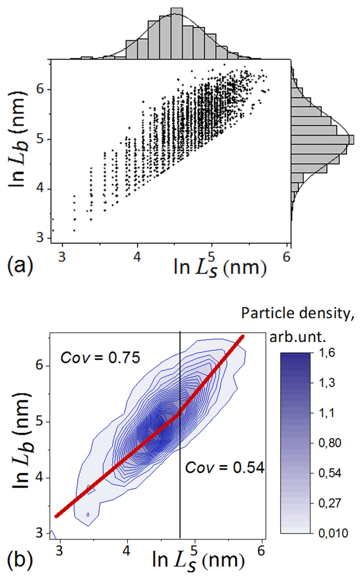
(a) Width Ls and length Lb of LiFePO4 particles. The corresponding frequency histograms are fitted with Lognormal functions. (b) Particle-density isolines for 5370 pieces with small sizes up to ln Ls = 4.8 (vertical line) and for 2030 large ones, the values of the covariance coefficients used in the calculations as a trial are indicated.
The XRD methodology developed in [25,26] and implemented in the MAUD software [27,28] was used for an anisotropic refinement of the crystallite size and strain values. X-Ray powder diffraction data were collected with a Bruker D8 Discover diffractometer operating in a parallel-beam linear-focus mode. The primary beam was conditioned with a double-bounce channel-cut Ge220. The Caglioti coefficients of the instrumental profile function were refined by fitting the data for a LaB6 powder. The values of L̄V[hkl] and of the errors, reported in Table 1 (in parentheses), characterize the reproducibility.

Mean XRD sizes L̄V[hkl] and the corresponding parameters of marginal Lognormal distributions L̄i, σi along the main crystallite axes, obtained by processing TEM measurements using the values of L̄V[hkl].
To divide the histograms of Ls, Lb into components and determine the required values of L̄i, σi, we use the values of L̄V[hkl] and the relationship between these: L̄V[010] < L̄V[100] < L̄V[001]. We assume that the probability of a crystal face to be aligned with the object plane of the microscope is proportional to its area. For example, the normalized probability for the (100) face is given by
The following assumption is that L̄b consists of two parts: one with the size L̄V[001] and the probability P(100)+P(010), and second with the size L̄V[100] and probability P(001). Similarly, L̄s consists of two parts: with the size L̄V[001] and the probability P (001) +P(010) and with the size L̄V[010] and probability P(100). The rationale for making these assumptions is contained in [17]. Further, assuming that large particles are blocky, we describe the histograms of L̄b and L̄s by Lognormal distributions with mean L̄V[001], L̄V[010] and L̄V[100], L̄V[010], respectively, we obtain the parameters of the marginal Lognormal distributions L̄i, σi (Table 1). To these parameters it is necessary to add the correlation coefficients rik, which have the following form, for example, for two arbitrary data arrays r12
In this way, full 3D Lognormal distributions can be obtained
where
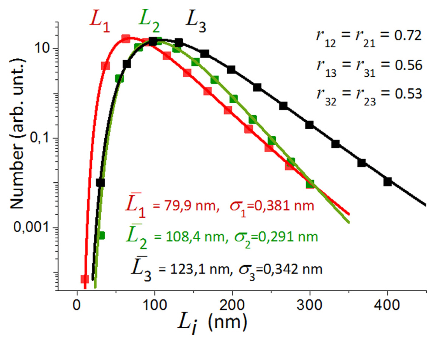
The results of fitting the parameters of a 3D 12-rank (12 points on each curve) discretization matrix of f(L̄) to the parameters of marginal distributions. The obtained correlation coefficient values are given.
Thus, the above second task has been solved, the parameters of 3D function f(L̄), described by equation (4) and including the correlation matrix with the parameters specified in Table 1 and in Fig. 4, were determined. Details of the program used are described in Supporting Information.
2.3 Electrochemical measurements of LiFePO4 cathodes
Electrodes were made, the active mass of which consisted of 80 wt.% powder, 10 wt.% acetylene black and 10 wt.% polyvinylidene fluoride (PVDF) and was applied as a homogenized suspension of the sample and acetylene black in a 5 wt.% solution of PVDF in N-methylpyrrolidone (analytical grade) on 1 cm2 aluminum plate, 0.4 mm thick, after which it was dried at 120°C in air for 12 hours. To reduce the errors of galvanostatic measurements of rate capability Q(t) at small t, the cathode thickness was minimal, about 8 μm (see Fig. 5).

SEM image of a side-cut LiFePO4 cathode. The sulfur structure of the LiFePO4 cathode is seen.
In addition, to reduce their porosity, the cathodes were subjected to multiple sequential rolling on V-6P-Yumo rolls. A sealed three-electrode cell with lithium deposited on a titanium plate as an auxiliary electrode and lithium as a reference electrode was used. The metallic Ti substrate does not show activity at potentials close to metallic Li, which excludes the formation of their alloy and was checked by us visually after completing numerous current experiments in the potential range of LiFePO4 electrodes. Ti oxidation is also not observed, which may be due to the presence of a thin passivation layer. Therefore, to improve contact of Li metal counter electrode with the current collector, a perforated Ti substrate with a deposited Li layer was used.
The schematic of the cell in application to our problem is illustrated in Supporting Information. By a half-cell we mean a cell whose polarizing circuit consists of the electrode under study (working electrode, in our case the LiFePO4 composite on aluminum plate) and the counter electrode (in our case the lithium metal on a perforated Ti substrate) [31]. The measuring circuit includes a separate third electrode. The material of this reference electrode in our case is also lithium.
The measurements included charge-discharge cycles with constant current loads: sequentially from 0.1 to 20 C in one cycle, then 15 cycles each, completing 10 cycles with a load of 1 C. The current density of 1 C corresponded to 170 μA per 1 mg of sample being analyzed at potentials in the range 2.6–4.3 V relative to the lithium reference electrode. The finished electrodes contained 1.5(3) mg of powder as part of the active mass distributed over the surface of Al plate with an area of 1.5–1.8 cm2. Fig. 6 shows the results of galvanostatic measurements.

(a) Galvanostatic charge-discharge curves and (b) variation of capacity with the cycle number. The values of the charge and discharge currents (C-units) are on the diagrams.
Cyclic voltammetry measurements were performed using the Autulab, EcoChem complex with an Autulab PGstate 202 potentiostat-galvanostat measuring unit. The potential sweep rate was from 0.05 to 10 mV/s in the potential range from 2.6 to 4.3 V relative to the lithium electrode. Before starting the potential sweep at the next speed, the tested electrode was kept at a potential of 2.6 V for 5 hours. The Fig. 7 shows the results of cyclic voltammetry measurements.
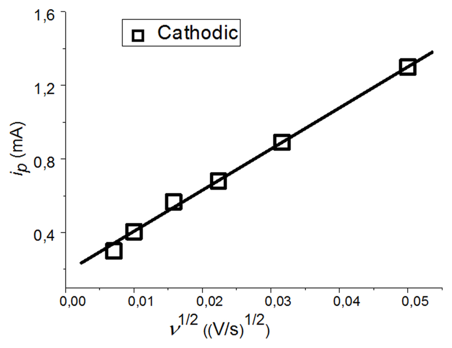
Dependence of cathodic peak currents on potential sweep rate.
The specific surface area of LiFePO4 powders was determined using an ASAP-2020 instrument from Micromeritics by adsorption-structural analysis. Degassing of the sample is carried out according to a given program, evacuation at 300°C for 10 hours, then measurement of the nitrogen adsorption and desorption isotherm at 77 K and calculation of the specific surface area of the sample using BET methods. A value of 23.1 m2/g was obtained.
3. Results and Discussion
3.1 Analytical model of rate capability Q (t)
To identify the dependence of the most important battery characteristics Q(t) on the particle shape of the initial cathode powders, on the function f(L̄) and its statistical parameters, we develop an analytical model using the following simplifications:
1. Important simplification is that the crystallite recharging is due to 1D Li diffusion along the M·dx2·dx3 column (see Fig. 1). By analogy with [8], to describe the rate capability qse(t) of a separate particle column shown in Fig. 1, we will use the following equation
where t is the time constant. In [8] the exponent values n are defined for batteries and supercapacitors, 0.5 and 1.0, respectively.
2. The main simplification is that equation (5) can be interpreted as the result of a probabilistic event [32], in which the rate capability qsu(t) is not realized with probability P in time t. That is, the event is described by the equation
As t → ∞, the probability P approaches 0, and q(t) asymptotically approaches the limit value qM. As t → 0, it approaches the dependence
3. According to [33], there are two types of equivalent circuits for electrochemical impedance analysis, shown in Fig. 8, parallel and series connection of circuits.
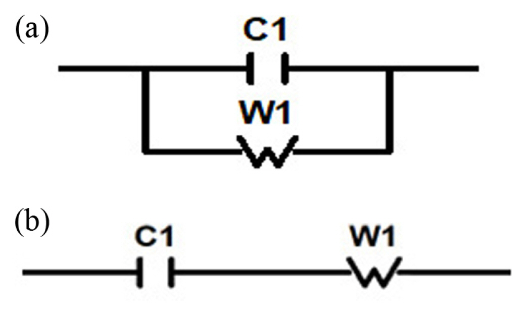
Equivalent circuits of (a) parallel and (b) series connection of capacitor C1 and Warburg element W1.
Fig. 8 can be compared with two probabilistic equations corresponding to the presence of parallelism or a sequence of events [32]
In this case, in equation (5) Warburg element described by diffusion time τd and capacitor described by the electrical time τel, both normalized to the discharge time t. An analysis of equations (5–8) makes it possible to draw the following 3 conclusions:
3.1 The parallel model does not correspond to the real experimental situation. Computer calculations have shown that as t decreases, a large slope in double logarithmic coordinates, about n = −1.5 (see Supporting Information), should be observed, which was not observed by us and rarely earlier in experiments [8].
3.2 The appearance of slope n = −1.5 is possibly due to experimental errors. To reduce the probability of this strong dependence in our experiments, the cathode thicknesses were minimally possible, and the large volumes of the electrochemical cell reduced cathode overheating under study at low t (high currents).
3.3 More realistic is the series model: lithium diffusion through the column and the presence of a double capacitor layer at its exit. In this case, the slope will be either −0.5 or −1.0 as t decreases, and ends with −1.5 at extremely small t.
4. Thus, for the rate capability column, we get the equation
The program used in this study (see Supporting Information) makes it possible, in principle, to set the complex dependence of D on the coordinate along the column M. The real mechanism of FePO4/LiFe-PO4 phase boundary motion [34–36] can be taken into account at least in a phenomenological way. In this study, the dependence
5. To describe the experimental rate capability Q(t) using the 3 D function f(L̄), we assume that it consists of the sum of the crystallite rate capabilities in the form qcr(t, L1, L2, L3), which can be obtained by integrating (9) over the volume of a crystallite with dimensions L1, L2, L3
where the limits of the first integration depend on the x3 coordinate.
Then (10) can be transformed into an N-bit 3D matrix
Thus, the above third task has been solved. The analytical model of rate capability Q(t) is developed, described by equations (9–11) and taking into account the anisotropic 3D distribution function of powder particles.
3.2 Determination of the experimental parameters of rate capability Q(t): D and tel
It should be noted that the analytical method used in [1–3] and chosen by us to describe the rate capability Q(t) are, in fact, phenomenological [39]. Especially the part described by equations (6–8) and associated with the use of probability theory. However, this developed analytical model does not yet correspond to the above-described task of studying mixed powders [16,22–24], including the LiFePO4 powder chosen by us. Therefore, to describe the mixture of cuboid and ellipsoidal particles shown in Fig. 2, we make the following phenomenological assumptions:
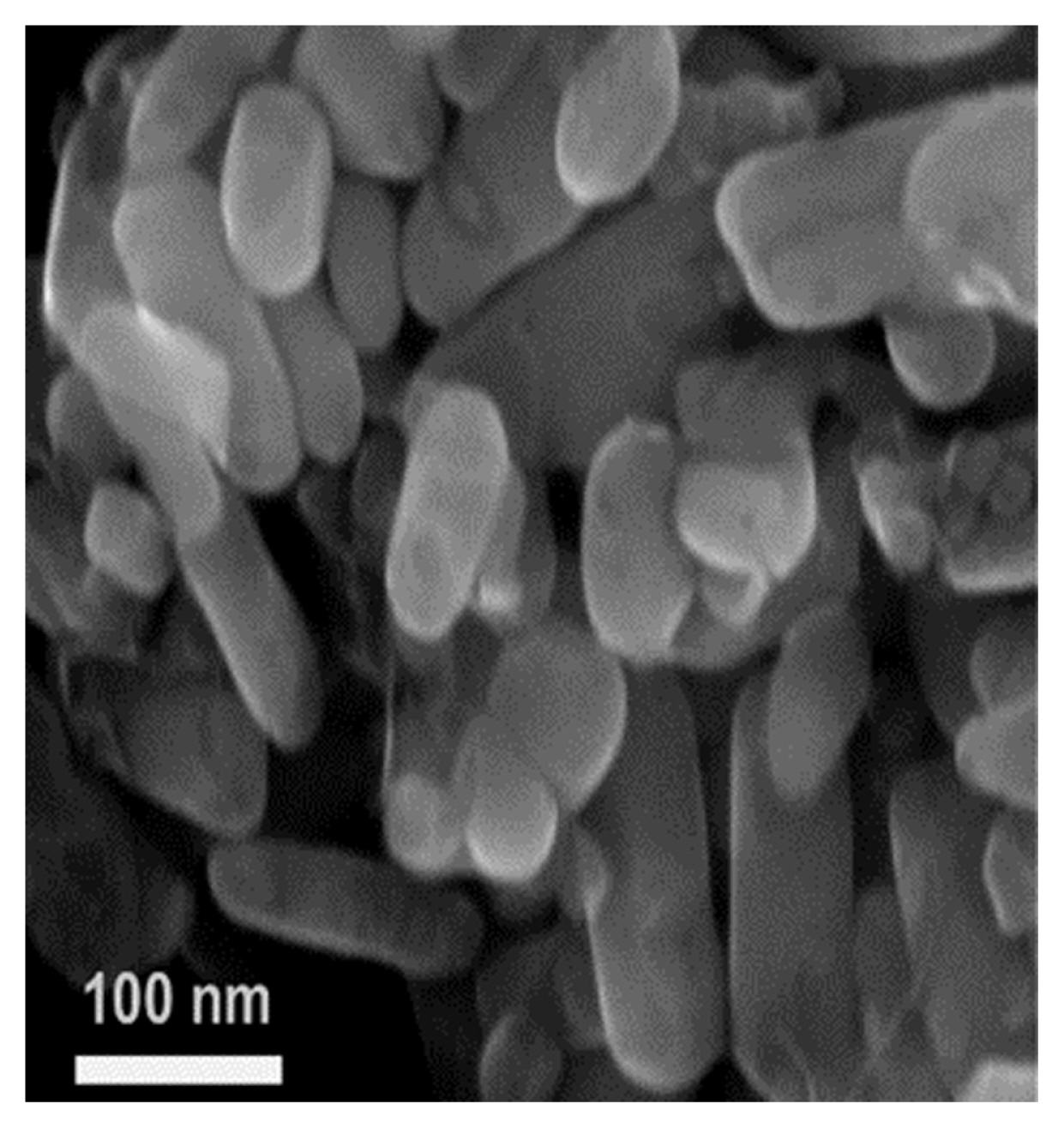
SEM image of the LiFePO4 powder particles. The larger ones are closer to the cuboid shape, and the smaller - to the ellipsoid shape.
1. We will use a normalization method similar to that described in [3]. Let us equate the value Q(tnr, D, τ), obtained using equation (11), with its experimental value Qnr(tnr) at the discharge tnr. That is, we consider
2. When describing complex analytic situations, a piecewise-continuous function is often used, which is joined at some intermediate value of the free parameter [40,41]. We assume that Q(t, D, τ) is piecewise-continuous at the point tnr. At t > tnr, it is determined by large particles and the parameters of the cuboid distribution function given in Table 1 can be used, and at t < tnr, it is determined by small ellipsoidal particles.
Using equation (11), a 3D N-rank matrix of capacity rate
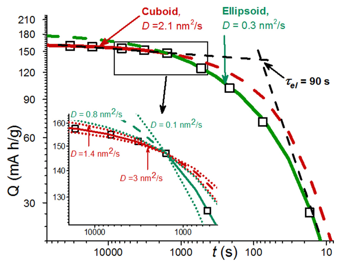
Fitting the theoretical dependences to the experimental measurements of the LiFePO4 cathode rate capability. Red lines - a cuboid model of crystallites, a solid line at long discharge times (tnr > 1800 s, < 2 C) and a dashed line, a continuation of the solid line, at small times, respectively. Green lines - an ellipsoidal model of crystallites, a dashed line at long discharge times (> 1800 s, < 2 C) and a solid line at small times, respectively. τel value approximately coincides with the time at the intersection point of the straight-line approximations (black dotted). The inset illustrates the dependence of the fitting accuracy on the values of the D.
Note that the unit of diffusion coefficient (nm2/s) we have chosen is more preferable, since it allows us to more clearly correlate D value with the particle sizes. For example, at D = 1 nm2/s, using the expression for the relaxation time for one-dimensional diffusion
Thus, the above fourth task has been solved. The adjustable parameter D is greater, by about 7 times, for large cuboid particles, D = 2.1 nm2/s, in comparison with small ellipsoid particles, D = 0.3 nm2/s. The value of D strongly depends on the particle discharge degree and can vary by 4 orders of magnitude [44], from 10−11 to 10−15 sm2/s (103–10−1 nm2/s). The value of obtained D is some averaging and is within this range. In this regard, it is important to compare them with other ways to get value of D, obviously also averaged, which, in particular, can be obtained as a result of galvanostatic measurements and using the Randles-Sevcik equation.
3.3 Comparison with the results of using the Randles-Sevcik equation
As can be seen from Fig. 7 the dependence of the magnitude of the cathode current peaks correspond to the applicability of the Randles-Sevcik equation, which at 25°C has the form
where ip - the peak current in amperes, constant 2.69 × 10⁵ with units of C/mol n 1/2, CLi - the initial concentration of Li in LiFePO4 in mol cm−3, taken as the total amount of Li in a particle before delithiation and is 0.0228 mol cm−3, n - potential sweep rate in V/ s, Sel - the electrode area in cm2, defined by us as the sum of the areas of the (010) planes of all cathode particles, D - diffusion coefficient in cm2/s [45,46]. Since the access of electrons to the particle must be ensured for the electrochemical reaction to take place, Li can escape from it only in one direction. That is why we assume that the particle interaction area is equal to the particle projection area on the (010) plane.
Next, the task is to find the value Sel. Using the weight of the powder in the cathode, 0.0015(3) g, and its density, 3.6 g/cm3, we can find the total volume of all cathode particles, Vexp= 4.2 × 10⁻⁴ cm3. On the other hand, similarly to (12), we find the average particle volume
where the size matrix f̄ is normalized to 1 in this case, v - matrix of particle volumes, each element of which has volume
As a result, we obtain areas Sel for cuboids and ellipsoids equal to 90 cm2 and 50 cm2 (specific surface 0.6 m2/g and 0.33 m2/g), respectively. These specific surface values are more than 1 order less than the BET value and almost 2 orders of magnitude greater than the area of the cathode electrode. Using Fig. 7 data, equation (13) and the values of Sel, we obtain diffusion coefficients of 0.9 nm2/s and 0.5 nm2/s in cuboid and ellipsoidal particles, respectively.
Thus, the above fifth task has been solved. Inconsistencies between the results of using the Randles-Sevcik equation with the results shown in Fig. 9 can be considered quite acceptable, since both methods of determining D have obvious sources of error. But the developed method has a clearly lower value of systematic errors due to the ability to really take into account the shape and statistics of crystallites, and it is also useful for improving the accuracy of the Randles-Sevcik equation.
3.4 Shape engineering of crystallites to optimize rate capability and increase the cathode capacity
To increase the capacity of LiFePO4 cathodes, efforts are mainly directed to the development of technology (shape engineering) to reduce the size of crystallites along the direction of Li diffusion, along the [010] axis. Some examples of LiFePO4 developments and studies of plate-like particles are shown in Table 2 [47–51], in which for [51] the results of 5 types of samples with different aspect ratio c/a (2.4–6.9) are briefly noted. The approach developed in our work makes it possible to quantitatively describe these and other technological experiments. First of all, let’s illustrate in Fig. 10 how the Lognormal distribution functions look like in double logarithmic coordinates. The statistical parameters hereinafter are close to the values obtained above in magnitude, and the dimensional parameters - are close to those occurring in Table 2.

Development and research of LiFePO4 plate-like particles
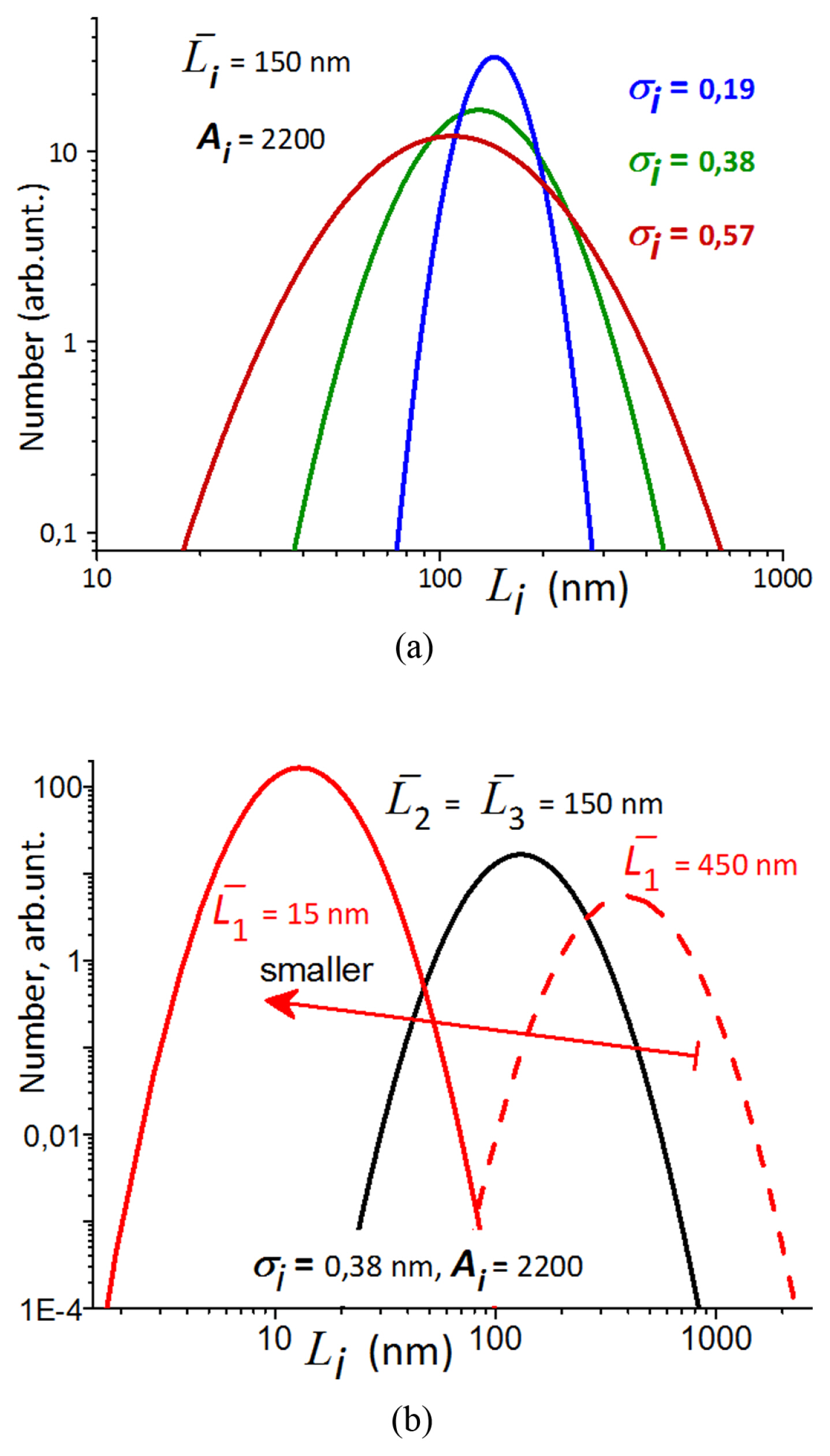
Lognormal distribution functions of crystallite sizes as a function of (a) dispersions and (b) their average values of L̄1. Examples of distributions of anisotropic particles to illustrate two extreme situations L̄1 « L̄2 = L̄3 and L̄1 » L̄2 = L̄3.
Thus, Lognormal distributions in the logarithmic x-coordinate look like a normal (Gaussian) distribution in the linear x-coordinate.
3.4.1 Task specification: need for rate capability rationing at small and big times
We specify the task as follows, dividing it into two subtasks:
1. Achieving a large rate capability (and capacity) at big times, or increasing the rate capability at small times, which can be solved by using shape engineering of crystallites.
2. Decreasing electrical relaxation time τel to increase the rate capability at small times, which is not directly solved by the technology of particles, but is necessary by improving the quality of their coating. Examples of this dependence will be given below, but in calculations it is sometimes assumed that τd » τel. We mean that τd is of the order of magnitude about minutes.
So, it is necessary to consider the conditions necessary to achieve maximum capacity values at large (> 0.05 C), and then at short (< 1 C) recharge times. To do this, we fix by software the values of the preexponential factors in the calculations Q1C = 135 mAh/g and Q0.01C = 170 mAh/g, respectively. (Sometimes other values will be used to better illustrate the Q(t) dependencies.) A similar principle of rate capability rationing, in other words, linking theoretical curves to experimental results, has already been used in equation (12) above.
Fig. 11 illustrates the rate capability, which are selected as a capacity of 135 mAh/g at a rate of 1C (t = 3600 s). It can be seen that an increase in rate capability at big times leads to its decrease at small times and vice versa. At t → ∞, rationing integration normalizations (11) and crystallite size distribution function (4), the quantity Q(t, Dif, τ), defined by equation (5), will be equal to the theoretical limit capacity LiFePO4 cathode Q0 = 170 mAh/g. This means that in some cases, in particular, in Fig. 11 for the parameters of the curve with average values of cuboid crystallites L̄1 = 300 nm, a region of times t > tcrt arises that is greater than some critical value tcrt, for which Q > Q0. This means that for these values of the dependence parameters, its inflection will occur at the point tcrt. If, for other parameters, the limiting values Q < Q0, it can be concluded that there are non-optimal stages in the powder technology with the presence of inactive impurities in them, or a slow approach of Q to its asymptotic value Q0.

An illustration of rate capability rationing. Average L̄1 size values are indicated, L̄2 = L̄3 = 150 nm, τ = 90 s, D = 2 nm2/s.
Thus, Fig. 11 shows that an increase in capacity at small times will inevitably lead to a decrease in capacity at big times, and an increase in capacity can only be achieved by reducing it at small times, i.e., by reducing battery power. Below, additional examples will be given that also confirm these conclusions.
3.4.2 Task specification
Influence of electrical relaxation time τel
Fig. 12 and 13 show the results of calculations for electrical relaxation time τel = 0.09 s and three orders of magnitude larger τel, respectively, for guaranteed fulfillment of the inequality τd » τel in the first variant. The ranges of coordinates are chosen so that the differences in the dependences of the curves on the values of the calculation parameters would be visually observable. In particular, it is seen that the slopes tangents of the falling dependence parts in Fig. 12a and 13a are close to −0.5 and −1.0, respectively. The inset of Fig. 12a highlights the results shown in Table 2, obtained in [47–51] and which were normalized to the value of rate capability at 0.1 C. The latter was done to equalize their possibly different quality of particle coverage.
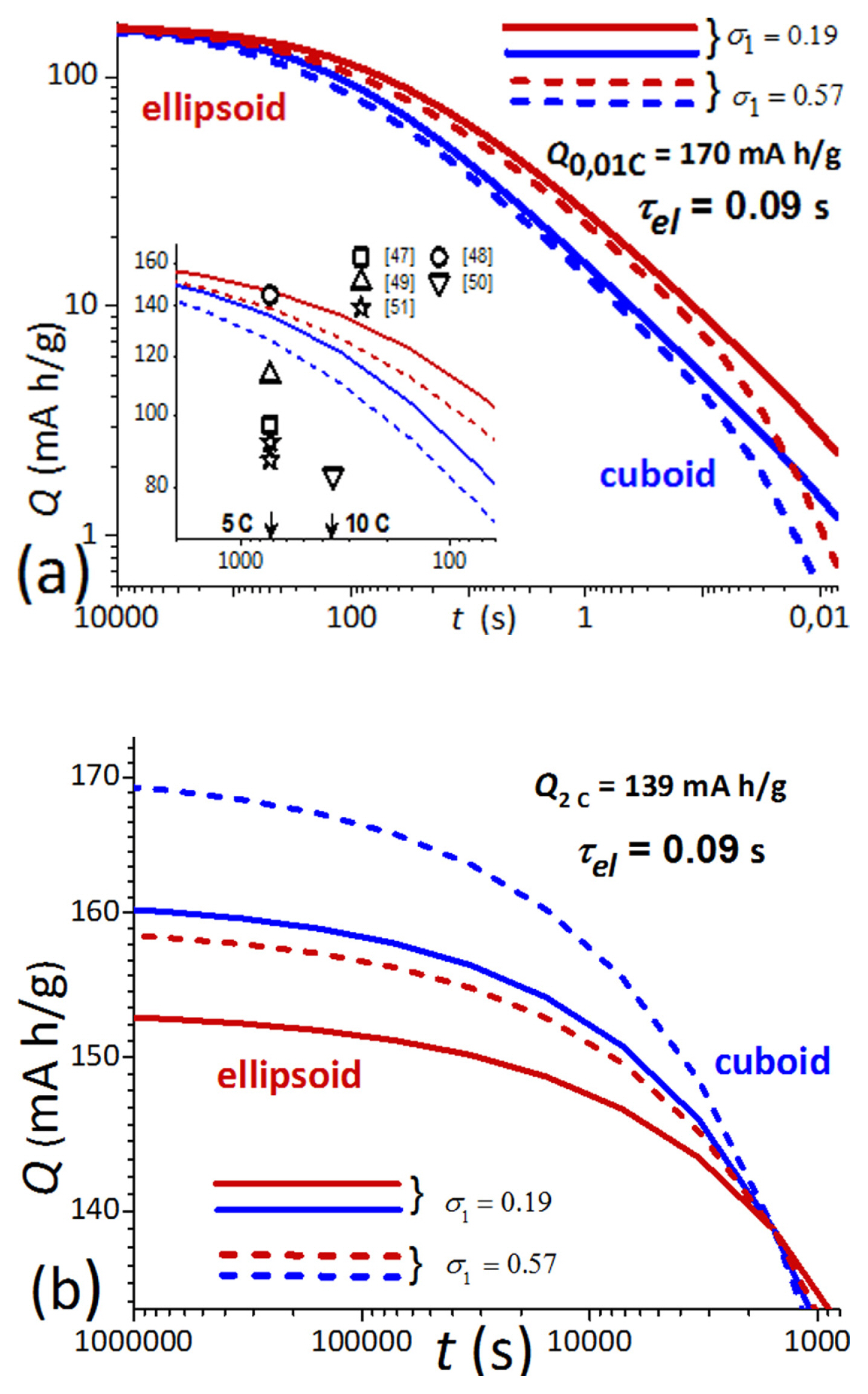

Rate capability for two dispersion values: 0.19 and 0.57, for cuboids and ellipsoids. (a) and (b) for relaxation times of 90 s and for rationing to values Q0,01C and Q2C, respectively. L̄1 = 75 nm, L̄2 = L̄3 = 150 nm, D =2 nm2/s.
Thus, from Fig. 12a and 13a it can be seen that if the theoretical limit of the capacity rate is reached for big times, then to increase it at small times. Powders of ellipsoidal crystallites, small dispersion of their size distributions and a small electrical relaxation are preferable. At the same time, it can be seen from Fig. 12b and 13b that if a certain specified value is reached for small times, for example, Q2C = 139 mAh/g, then opposite parameter changes are needed to increase rate capability at big times. In particular, cuboid-shaped crystallite powders with large dispersion of their size distributions are preferable and the magnitude of the electrical relaxation time is insignificant.
3.4.3 Influence of covariances
Previously, the influence of the correlation between the sizes of crystallites and the correlation matrix as a whole on the parameters of electrochemical current sources was not discussed. Fig. 14a shows a part of the title Figure (Novelty), and in Fig. 14b continuation of these dependences into the region of small times < 3600 s (> 1 C), namely, at t = 360 s.
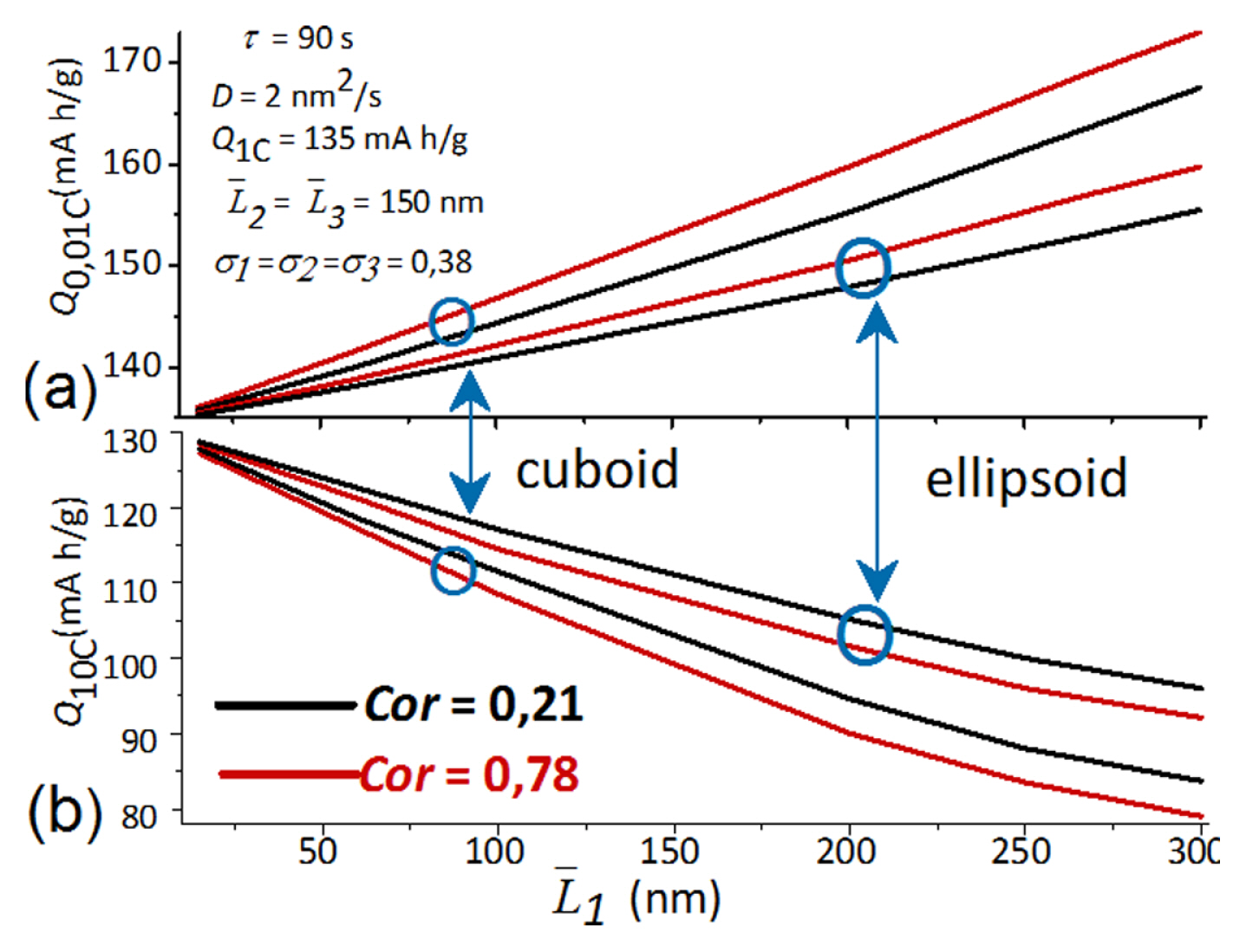
Dependence of the rate capability at low and high rates: (a) Q0,01C and (b) Q10C. On the shape of crystallites, their average size along the [010] axis and other parameters of their distribution statistics, presented here.
Thus, as can be seen from Fig. 14, increase in rate capability can only be achieved by reducing it at small times. In this case, the change in the correlation coefficient is significant, but does not allow us to combine the requirements for its simultaneous increase in the region of small and big times. That is, there is also an incompatibility of requirements for obtaining maximum capacity and maximum rate capability.
3.4.4 Influence of size along the [010] axis
In [48], a 5-fold increase in the rate capability of LiFePO4 cathodes was achieved, and in [50], its 6-fold increase was achieved with a decrease in the particle size along the [010] direction of diffusion of lithium ions. Fig. 15 shows calculations using the distributions shown in Fig. 10. It can be seen that such a multiplicity can be achieved and is strongly dependent on the value of the diffusion coefficient. To a much lesser extent, the dependence on the shape of particles is manifested in comparison with the experimental dependence Fig. 9. This is due to the following calculation feature. In Fig. 15, the same values of statistical parameters are used, in particular, the average particle sizes along 3 crystallographic axes. The dimensions of Fig. 9 are different, shown in Table 1 and obtained as a result of the described features of processing real XRD measurements.
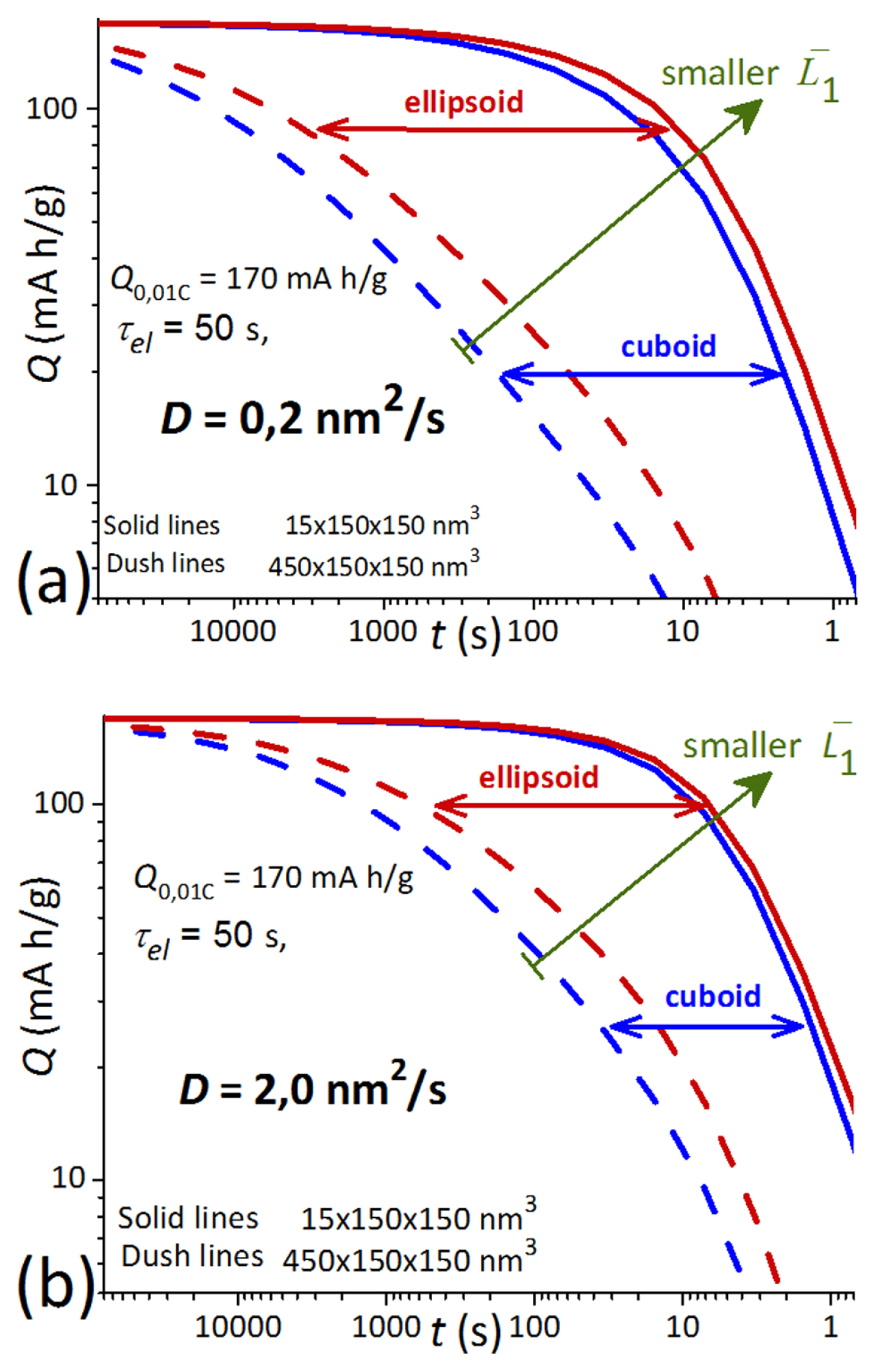
Rate capability dependences for the two extreme ratios between the parameters of the average crystallite size along the [010] axis, shown in Fig. 10(a) and (b) for different D values indicated in the figures, other parameters are identical.
Thus, the dependences of the rate capability on the crystallite size along the [010] axis for L̄1 = 15 nm and = 450 nm with the parameters of the correlation matrix close to the experimental are shown in Fig. 15. This dependence turns out to be significant for small values of D and cuboid crystallite shapes. The Supporting Information contains additional calculations on the influence of the D, τel and particle face area (010) on the rate capability.
4. Conclusions
We demonstrate a correspondence between the crystallite anisotropic sizes of LiFePO4 powder: between the averaged over the crystallite columns L̄i XRD, obtained from XRD measurements, and averaged over the volume L̄i TEM, obtained from TEM measurements, which for Lognarmel distributions can be related to the average sizes of real measurements L̄i. In this way, a full 3D Lognormal distribut ion function can be obtained, including its correlation matrix of the distribution between the crystallite sizes in their three crystallographic directions.
A LiFePO4 powder was chosen for testing the developed model, consisting of big cuboid and small ellipsoid crystallites. Bearing in mind that the study of such mixed powders, although a difficult task, is very important in connection with a promising technological direction in which a denser electrode mass is achieved by mixing particles of various sizes. In this case, smaller particles are located in the voids between large ones. To reduce the errors of galvanostatic measurements of rate capability Q(t) at small t, the cathode thickness was minimal, about 8 μm.
The analytical model of rate capability Q(t) is developed, described by equations (9–11) and taking into account the anisotropic 3D distribution function of powder particles. The main model simplification is that electrochemical processes are described as probabilistic events, in which the rate capability of the crystallite column qsu(t) is an event and is realized with probability (1–P) dependent on time t. That is, the event is described by the equation q(t) = qM(1 – P), and at t → ∞ the probability P → 0, in particular.
To be able to apply the developed analytical model for experimental parameters determination of mixed powder rate capability Q(t) (D and τel), the following important simplifications have been made. We assume that Q(t, D, τ) is piecewise-continuous with some intermediate point tnr. At t > tnr, it is determined by large particles and the parameters of the cuboid distribution function given in Table 1 can be used, and at t > tnr, it is determined by small ellipsoidal particles.
It turned out that the parameter D adjusted to the experimental dependence is greater, by about 7 times, for large cuboid particles, D = 2.1 nm2/s, in comparison with small ellipsoid particles, D = 0.3 nm2/s. These values are within the limits usually obtained earlier, but then they were compared with the values obtained as a result of galvanostatic measurements of the test sample and using the Randles-Sevcik equation. On this path, the area of the electrodes Sel was determined, defined as the sum of the areas of the (010) planes of all cathode particles. So, we obtain diffusion coefficients of 0.9 nm2/s and 0.5 nm2/s in cuboid and ellipsoidal particles, respectively. Inconsistencies between those results with the results of the developed method can be considered quite acceptable.
Task of crystallite shape engineering to optimize the rate capability and increase the cathode capacity can be specified as follows, dividing it into two subtasks:
Achieving a large rate capability (and capacity) at big times, or increasing the rate capability at small times.
Decreasing electrical relaxation time τel to increase the rate capability at small times, which is not directly solved by the technology of particles, but is necessary by improving the quality of their coating.

Supporting Information
Some details of the measurement technique, the developed program, the possibilities of its use to optimize the technology of electrode powders are given in Supporting Information, available from the article site or from the author.
Acknowledgement
XRD studies were performed in Resource Center of St. Petersburg State University. SEM studies were partly performed in Collective Use Center “Materials Science and Diagnostics in Advanced Technologies”, TEM in the Omsk Center for Collective Use. Half of the work done at the Ioffe Institute.
AV Ushakov and AV Ivanishchev participate in RSF 21-73-10091 and RFBR 20-03-00381 grants, respectively.