Conversion of a Constant Phase Element to an Equivalent Capacitor

Byoung-Yong Chang

doi:10.33961/jecst.2020.00815

Abstract

Here I present a formula which converts a constant phase element (CPE) to its equivalent capacitor. Electrochemical impedance spectroscopy is capable of resolving a complex electrochemical processes into its faradaic and non-faradaic elements, and the non-faradaic process is frequently described as a CPE in place of a capacitor due to the non-ideality. Being described as a capacitor, the non-faradaic element provides information by its capacitance, but a CPE cannot provide a physical meaning. In order to solve the problem, the CPE has been dealt with as an equivalent capacitor of which the capacitance provides practical information. Succeeding the two methods previously suggested, a new conversion method is suggested in this report. While the previous ones manipulate only the CPE, the new method takes both the CPE and its related resistor into account for conversion. By comparing the results obtained by the three methods, we learn that the results are nearly the same within tolerable ranges, and conclude that any of the method choices is acceptable depending on the conditions of the system of interest.

Keywords: Electrochemical Impedance, Constant Phase Element, Nyquist Plot

1. Introduction

Electrochemical impedance spectroscopy is the only electrochemical measurement technique which can resolve electrochemical processes into faradaic and non-faradaic components. Generally, an electrochemical process consisting of a faradaic and a non-faradaic components is described as an equivalent circuit consisting of a resistor and a capacitor connected parallelly [1]. It is obvious that a faradaic process can be characterized as a resistor because charges are transferred directly during the process, but it is vague to designate a non-faradaic process to a specific component. When an electrode is polarized, charges are accumulated at the electrode/solution interface of which the medium is dielectric material to drive formation of an electric double layer. As a result of that, a non-faradaic process is mostly designed as a capacitor. Not only that, adsorption of charged molecules in the electrolyte medium and a delayed response of a faradaic reaction also show capacitive effects [2–4].

Even though such a non-faradaic component is expected to be presented as an ideal capacitor, the practical observation results in non-ideal behaviors of a capacitor; while an ideal capacitor shifts electric signals by the phase of π/2, the practical signals are measured being shifted by n·π/2 where n is given between around 0.8 to 1. Owing to the phase shift by a certain degree, the element is called a constant phase element (CPE) that also includes a normal capacitor when n = 1, and its impedance is expressed below [5],

eq (1)

ZCPE=1Y0(iω)n

where ω is angular frequency, Y₀ and n are the characteristic parameters of the CPE. Therefore, instead of a capacitor, a CPE is very frequently used in analysis of electrochemical impedance spectrum in many practical cases [6–9].

A CPE definitely results in a better fitting curve than a capacitor, but its parameter, Y₀, does not give clear physical meaning as capacitance does. Over this problem, E. van Westing suggested a formula to convert Y₀ to an equivalent capacitance [10].

eq (2)

C=Y0(ω)n-1sin(nπ/2)

Then, many scientists proposed practical applications of the above formula to real systems. Again, C. H. Hsu and F. Mansfeld suggested an advanced conversion method in their technical note [11].

eq (3)

C=Y0(ωmax″)n-1

with ωmax″ is the frequency where the imaginary part of impedance has its maximum.

Here I present another conversion method developed from a different approach. The two well-known method try to calculate the capacitance only using the imaginary part of impedance, but the new method uses both the imaginary and real parts of impedance interfered by the CPE. As a result, we can find the effective capacitance and resistance for the parallel circuit consisting of a constant phase element and a resistor.

2. Theory and Simulations

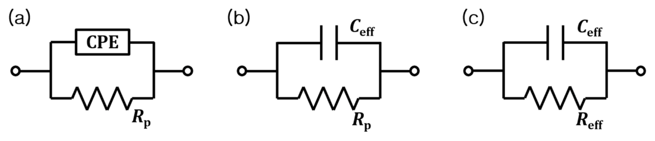
In order to find an equivalent capacitance of a CPE, the circuit of a resistor (R_p) and a CPE in Fig. 1(a) needs to be modified to another equivalent circuit consisting of a resistor and a capacitor in parallel. The conversion methods of eq (2) and (3) are based on the assumption that the CPE only affects the imaginary part of impedance, and build the equivalent circuit in Fig. 1(b). However, as the impedance of a CPE in eq (1) is rearranged to 1Y0ω-n(cos(nπ2)-isin(nπ2)), the real part of impedance should be accounted in the modified circuit. Therefore, we can set up another circuit of which the CPE and the Rp are replaced with a C_eff and a R_eff as shown in Fig. 1(c).

It is already known that a CPE can also be described by distribution of time constants and has electrical impedance expressed by the equation below [12],

eq (4)

Z=Ro[1+(iωT)n]

where T is the time constant for the decaying current and R₀ is a resistor. Here, we can infer that the decaying current is rendered by the capacitive element which is parallelly connected to a resistor, which leads to the distributed time constant to be defined as

eq (5)

T=Ceff·Reff

As the impedance of the circuit in Fig. 1(a) is expressed below

eq (6)

Z=Rp[1+(iω)nY0Rp]

and should yield the same impedance results of eq (4), the following equation is derived.

eq (7)

T=(Y0Rp)1/n=Ceff·Reff

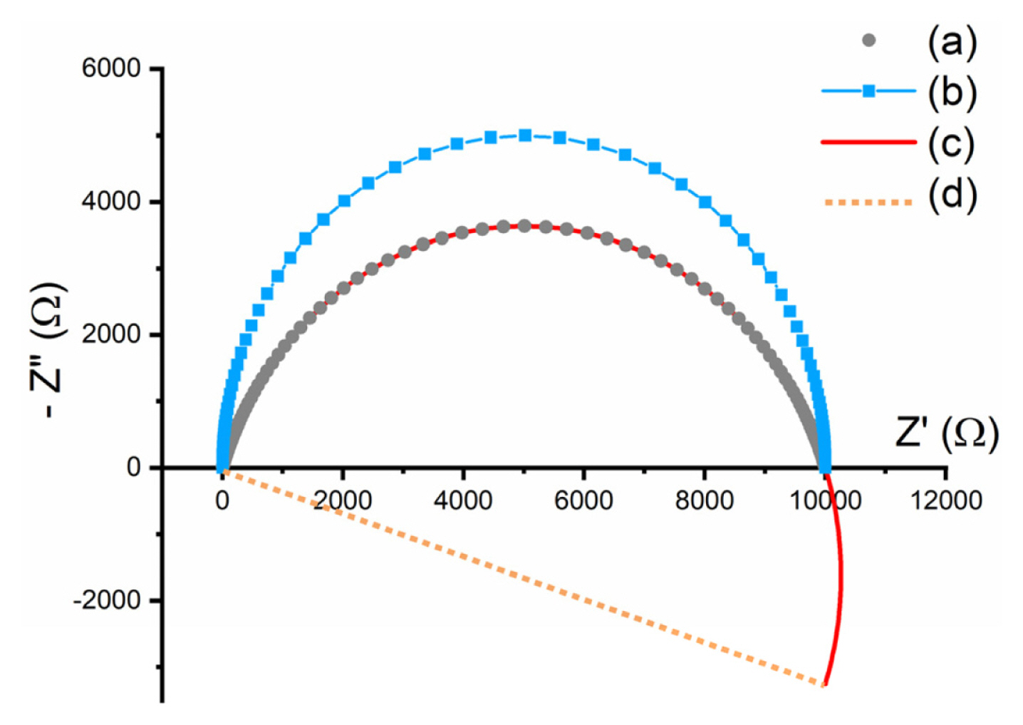
Fig. 2 shows Nyquist plots for the circuit in Fig. 1(a) with n = 0.8 (a,

) and 1 (b,

). Plot (b) shows the same semi-circle of the Nyquist plot of the circuit in Fig. 1(b) having an equivalent capacitance converted from Y₀ by eq (2) or (3). While Plot (b) with n = 1 shows a perfect semi-circle, Plot (a) with n = 0.8 does a depressed semi-circle. Even though the semicircle of Plot (a) looks depressed, it should be a perfect semi-circle if the circuit has a capacitor and resistor in parallel. So, the circuit of Fig. 1(a) can be re-designed to that of Fig. 1(c). The perfect semi-circle can be found when it is made with

eq (8)

Reff=Rp/sin(nπ2)

and transformed by the factor of (cos(nπ2)-isin(nπ2)), which is drawn in red (c,

). The curve is a perfect semi-circle extending the depressed semi-circle. With eq (8) plugged into eq (7), the effective capacitance can be obtained as below,

eq (9)

Ceff=(Y0Rp)1/nRpsin(nπ2)

The physical meaning of the rotation is not yet clearly explored as the physical meaning of n of a CPE is still controversial. But the rotation of the semi-circle can be comparable to depression of the semi-circle. A full rotation corresponds to no depression with n = 1 while partial rotations do to partial depressions of the semi-circle with n less than 1.

3. Results and Discussion

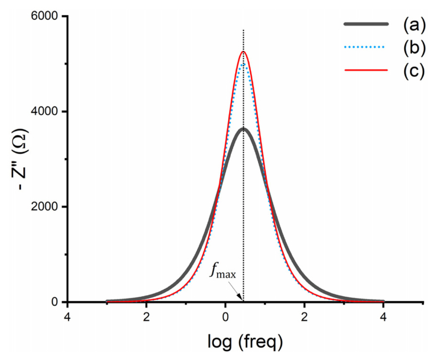
Simulations for impedance spectrum are carried out for the three equivalent circuits in Fig. 1 with converted values obtained by the methods of Westing [10], Hsu [11] and this report; the simulation conditions are R_s = 1 Ω, R_p = 1×10⁴ Ω, Y₀ = 1×10⁻⁵ sⁿ/Ω and n = 0.8 to 1. In order to compare the methods, we should discuss about two observations on the imaginary number of the impedance (-Z″) vs. log(frequency) shown in Fig. 3. One is that all the maximum numbers are found at the same frequencies, f_max, which confirms the equivalency of the circuits as shown by the results in the literature [11]. The other one is that the values are different along the frequency, which is explained in terms of resistance. The integration method enables to theoretically calculate the resistance using the following equation [13],

eq (10)

R=(9.2π)(∫∞fmaxZ″)dlogf

and the calculation result exactly matches to R_eff, which also confirms that a parallel connection of a CPE and a R_p can be described as that of a C_eff and a R_eff. The results of the converted capacitances for different n values are summarized in Table 1, and compared by methods using eq (2) and eq (3). The values are learned to be nearly the same within tolerance of 3% for n = 0.9 corresponding to a usual case and even 9% for n = 0.8 corresponding to extreme cases.

4. Conclusions

In analysis of electrochemical impedance spectra, the capacitive component is usually observed to have a non-ideal behavior and described as a constant phase element (CPE) of which the parameters are Y₀ and n instead of the conventional capacitance, C. While capacitance is clearly defined to have physical meaning, Y₀ is ambiguously known. Nevertheless, it is still considered to be analogous to capacitance, and has been studied to have a physical quantity equivalent to capacitance. To that purpose, two formula are already suggested and used widely. On the extension of the development, in this report, another formula is suggested with a different approach. In this approach, a decaying current generated by a CPE and a resistor is equivalently described as the one by an effective capacitor and an effective resistor, so that the current should have a time-constant. The time constant is related to Y₀ and n which lead to the values of the effective capacitor and resistor simultaneously. While the previous two methods only consider Y₀ and n of the CPE, the new one takes the effective resistance into account for the conversion process.

Among the three formulae suggested, which will give the most accurate result? The choice does not have to be worried about because there does not exist the exact value. A CPE holds both nature of capacitance and resistance which are dependent on frequencies, and the values are only estimated equivalently based on conditional assumptions. As a matter of fact, the values obtained by those methods are as slightly different as no significance is considered in the practical measurements. Any formula can be chosen depending on the conditions of the system of interest.

n	Calculated Capacitance (F/cm²)

	eq (2)	eq (3)	new
1	1.00×10⁻⁵	1.00×10⁻⁵	1.00×10⁻⁵
0.95	0.89×10⁻⁵	0.89×10⁻⁵	0.88×10⁻⁵
0.9	0.78×10⁻⁵	0.77×10⁻⁵	0.76×10⁻⁵
0.85	0.69×10⁻⁵	0.67×10⁻⁵	0.65×10⁻⁵
0.8	0.59×10⁻⁵	0.56×10⁻⁵	0.54×10⁻⁵