Effect of Zinc Addition in Filler Metal on Sacrificial Anode Cathodic Protection of Fin-Tube Aluminum Heat Exchanger

Yoon-Sik So; Eun-Ha Park; Jung-Gu Kim

doi:10.33961/jecst.2023.00374

J. Electrochem. Sci. Technol > Volume 14(4); 2023 > Article

So, Park, and Kim: Effect of Zinc Addition in Filler Metal on Sacrificial Anode Cathodic Protection of Fin-Tube Aluminum Heat Exchanger

Research Article

Journal of Electrochemical Science and Technology 2023;14(4):349-360.

Published online: September 15, 2023

DOI: https://doi.org/10.33961/jecst.2023.00374

Effect of Zinc Addition in Filler Metal on Sacrificial Anode Cathodic Protection of Fin-Tube Aluminum Heat Exchanger

Yoon-Sik So, Eun-Ha Park, Jung-Gu Kim^*

School of Advanced Materials Science and Engineering, Sungkyunkwan University, Suwon 16419, Korea

^*E-mail address: kimjg@skku.edu

Received May 16, 2023 Accepted August 2, 2023

This is an open-access article distributed under the terms of the Creative Commons Attribution Non-Commercial License (http://creativecommons.org/licenses/by-nc/4.0) which permits unrestricted non-commercial use, distribution, and reproduction in any medium, provided the original work is properly cited.

Abstract

This study investigated the tri-metallic galvanic coupling of different metals in the tubes, fillers, and fins of a heat exchanger. The goal was to prevent corrosion of the tubes using the fin as a sacrificial anode while ensuring that the filler metal has a more noble potential than the fin, to avoid detachment. The metals were arranged in descending order of corrosion potential, with the noblest potential assigned to the tube, followed by the filler metal and the fin. To address a reduction in protection current of the fin, the filler metal was modified by adding Zn to decrease its corrosion potential. However, increasing the Zn content of filler metal also increases its corrosion current. The study examined three different filler metals, considering their corrosion potential, and kinetics. The results suggest that a filler metal with 1.5 wt.% Zn addition is optimal for providing cathodic protection to the tube while reducing the reaction rate of the sacrificial anode.

Keywords: Aluminum alloy, Heat exchanger, Galvanic corrosion, Computer simulations, Electrochemical impedance spectroscopy

1. Introduction

Heat exchangers constitute a critical component of energy-related installations for heat management [1–3], and the increasing demand for energy conservation [4] drives the need for high-efficiency heat exchangers. Various methods have been proposed to enhance heat exchange efficiency, including increasing the surface area [5,6], improving heat transfer [7,8], and fluid control [9]. However, even the most efficient heat exchanger may suffer from reduced efficiency if it malfunctions due to corrosion [10]. Thus, improving the corrosion resistance of heat exchangers can increase their efficiency by extending their lifespan [11,12]. The fin-tube Al heat exchanger, consisting of three metals (fin, filler metal, and tube), is commonly used in home appliances and vehicles [13]. The use of dissimilar metals is necessary due to the different mechanical properties required for each part of the heat exchanger [14,15]. A tri-metallic galvanic couple is formed when the heat exchanger is exposed to corrosive environments [16–18]. Galvanic corrosion is a highly localized form of corrosion that can significantly reduce the lifespan of a product when in contact with other metals [19,20]. However, this phenomenon can also be used to extend the lifespan of a heat exchanger by applying sacrificial anode cathodic protection (SACP) which uses the fin as the sacrificial anode. Therefore, to improve the lifespan of fintube Al heat exchangers, research effort has been aimed at determining the corrosion potential of Al alloys [21]. Previous studies have observed that using filler metal with more active corrosion potential than Al tube alloy is preferable. Therefore, Zn is added to the filler metal [22]. However, increasing the Zn content of the Al alloy also increases the corrosion current density of the filler metal [23,24], which can affect the corrosion behavior of the Al heat exchanger in the tri-metallic galvanic couple [25]. Therefore, it is essential to investigate the effect of corrosion current density when designing SACP. Although many studies on SACP have focused on the corrosion potential [26–30], there is a lack of research on corrosion current density. Thus, in this study, we aim to enhance the lifespan of heat exchangers by considering both corrosion potential and corrosion current density, which will be based on the Butler-Volmer equation and mixed potential theory [31]. To achieve this objective, the galvanic coupling for SACP of 3xxx series Al alloy tube and fin material with three 4xxx series filler metals, each with varying Zn content, were evaluated. Scanning electron microscopy (SEM) with energy dispersive X-ray spectroscopy (EDS) was employed to analyze the microstructure of the filler metals. Additionally, to evaluate the effect of the filler metal on corrosion properties, both a potentiodynamic polarization test and electrochemical impedance spectroscopy (EIS) were conducted. Lastly, a galvanic corrosion simulation was performed to verify the effect of SACP, considering the ratio of area, geometric shape, and electrochemical properties for candidate metals [32,33].

2. Experimental

2.1 Specimens and solution preparation

The fin material, made of an Al alloy, was cast into a rectangular shape with its composition controlled using AA3003 and Al–20Zn master alloy. To reduce the corrosion potential of the fin, 2.5 wt.% Zn was added. The tube materials, which was UniCorAl^®, U3003 [34], was also cast into a rectangular shape, with its composition controlled using master alloys such as Al–20Mn and Al–15Zr. For the filler metals, rectangular ingots were cast using Al alloys, and their composition was controlled with master alloys such as Al–10Si and Al–20Zn. To evaluate the effect of the filler metal on SACP, 0.5 wt.% to 2.0 wt.% of Zn were employed. Table 1 presents the chemical compositions of the Al alloys used for the heat exchanger. All the alloy ingots were cut into a cuboid shape measuring 100 mm × 80 mm × 8 mm, and cold rolling was performed with thickness 30%, 60%, and 80% thickness reduction. Finally, the cold-worked specimens were cut into 15 mm × 15 mm × 2 mm for electrochemical test. The corrosion properties of the alloys were evaluated in seawater acetic acid test (SWAAT) solution at 49?, which contained 5 wt.% NaCl in deionized water and had its pH adjusted to 3 using an acetic acid solution (ASTM G85) [35].

2.2 Microstructural analysis

The microstructure of the filler metals was examined using an SEM (S-3000H, Hitachi, Tokyo, Japan). Before the analysis, the specimens were mechanically polished with silicon paper ranging from 600-grit to 2000-grit. Subsequently, the specimens were polished to microscale using 0.5 μm alumina suspension. Finally, the surface of the specimens was rinsed with ethanol and distilled water before being dried with nitrogen.

2.3 Electrochemical tests

The electrochemical behavior of the Al alloys was evaluated with a multi-potentiostat/galvanostat (VMP-2, Bio-Logic Science Instruments, Seyssinet-Pariset, France) using a three-electrode cell. The working electrode had each Al alloy, the counter electrode comprised two pure graphite rods (Qrins, Seoul, Korea), and the reference electrode consisted of a saturated calomel electrode (Qrins, Seoul, Korea). Before conducting the electrochemical tests, the specimens were abraded with 600-grit silicon carbide paper. Furthermore, the specimen was covered with silicone rubber, leaving an area of 1 cm² to regulate the reaction area. The open-circuit potential (OCP) was recorded for 12 hours until the specimen had an electrochemically stable surface. Following the OCP measurement, polarization tests were conducted at a potential sweep of 0.166 mV/s from the OCP to −0.25 V versus the OCP for the cathodic polarization and from the OCP to +0.50 V versus the OCP for the anodic polarization. EIS tests were performed under OCP with a sinusoidal amplitude of 10 mV in the frequency range from 100 kHz to 10 mHz. An equivalent circuit was applied to the EIS test results, and the outcomes were analyzed through an appropriate fitting process using ZSimpWin software based on the equivalent circuit.

2.4 Modeling and boundary conditions

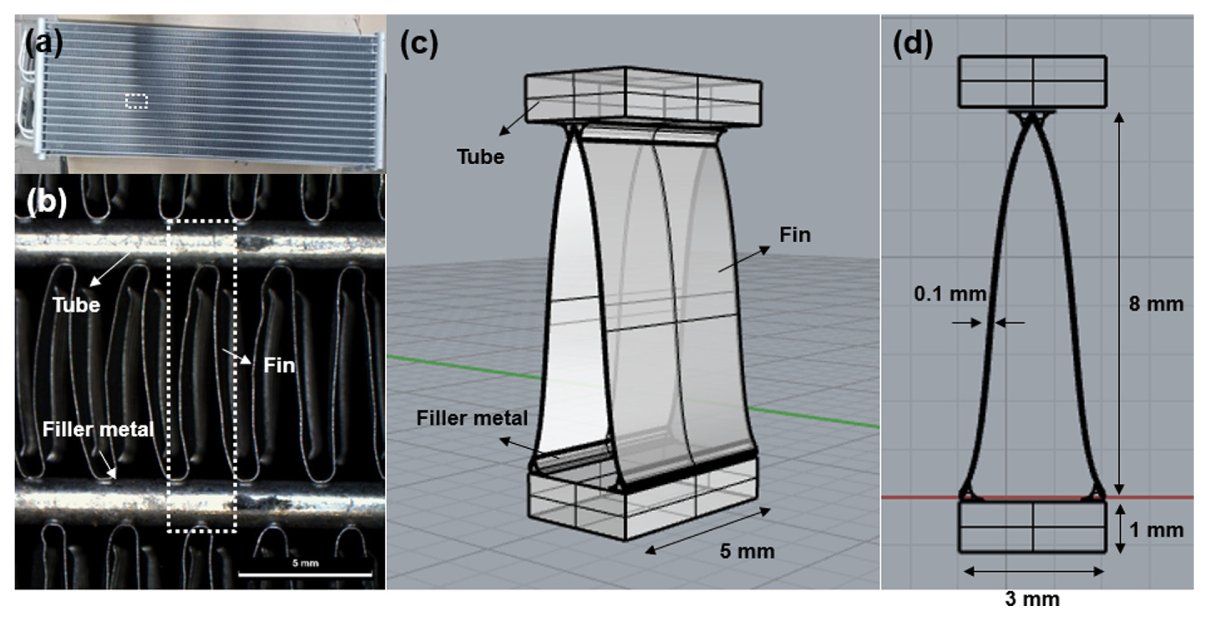
As presented in Fig. 1, a 3D heat exchanger model was designed using Rhinoceros 7.0 (Robert McNeel & Associates, Seattle, USA) based on the actual shape and dimensions. Table 2 provides the detailed dimensions of the 3D model. To simplify the heat exchanger model, the filler metal part was modeled with a triangular prism shape located between the tube and fin. The areas of the tube, filler metal, and fin were 92, 6.36, and 166 mm², respectively.

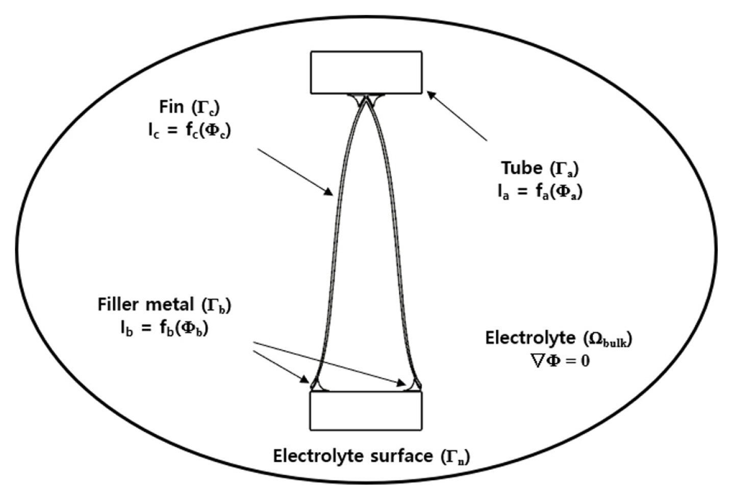
After modeling, the 3D model was imported into BEASY software (BEASY Ltd., Southampton, England) for galvanic corrosion simulation. The numerical simulations were conducted based on the corrosion properties of the filler metal. This simulation assumed that the model was completely immersed in the solution. Fig. 2 depicts the simulation model and boundary conditions, where the boundary condition was electrolyte domains (Ω), encircled by the surfaces of the electrolyte (Γ_n), the surfaces of the tube (Γ_a), the surfaces of the filler metal (Γ_b), and the surfaces of the fin (Γ_c) [36]. The electrolyte conductivity (σ) was consistent over the entire domain, and no current loss was assumed. The potential field in the electrolyte domain was modeled using the Laplace equation as follows [37]:

(1)

∇2Φ=0

where Φ is the electrical potential relative to the reference electrode.

The Laplace equation is solved using the following boundary conditions:

(2)

i=i0, on Γn

(3)

ia=fa(Φa), on Γn

(4)

ib=fb(Φb), on Γb

(5)

ic=fc(Φc), on Γc

where i₀ is the current density at any point inside the electrolyte. f_a(Φ_a), f_b(Φ_b), and f_c(Φ_c) are nonlinear functions on each surface representing the polarization behavior of each part. The current over the entire surface could be calculated based on this.

3. Results and Discussion

3.1 Microstructure and precipitate analysis

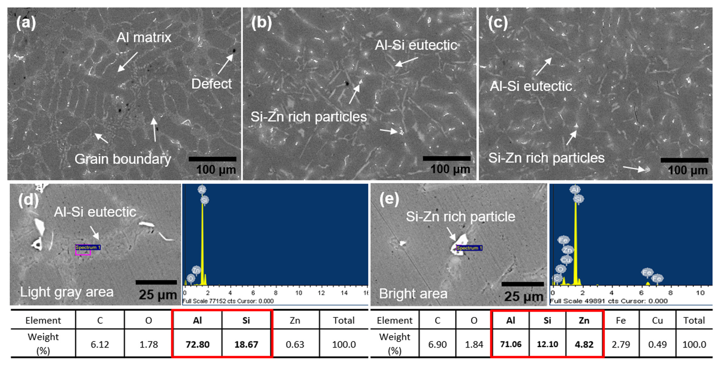
Fig. 3 presents the SEM images and EDS analysis of the filler metals without etching. The filler metals exhibited casting defects due to gas adsorption, Al oxidation, and precipitates along the grain boundary. The main elements of the filler metal alloy are Si and Zn. Si was added to lower the melting temperature of the alloy for brazing [38,39], whereas Zn was added to improve the efficiency of the SACP of the fin by lowering the corrosion potential of the filler metal [19,22,40]. The added elements in the filler metal (Si and Zn) may be in the solid solution or isolated particles of a second phase, intermetallic compounds, or inclusions. Therefore, Si and Zn precipitated near the grain boundary during the casting process [41]. The images presented in Fig. 3(a–c) display the segregation enriched in the Si and Zn precipitates at the grain boundaries. Additionally, the EDS analysis in Fig. 3(d) indicates that the light gray region corresponds to the Al–Si eutectic near the grain boundaries [42,43]. The EDS result in Fig. 3(e) reveals that the bright region represents the Si- and Zn-rich precipitates along the grain boundaries [44], while the dark gray areas correspond to the Al matrix.

3.2 Corrosion behavior

3.2.1 Tube and fin materials

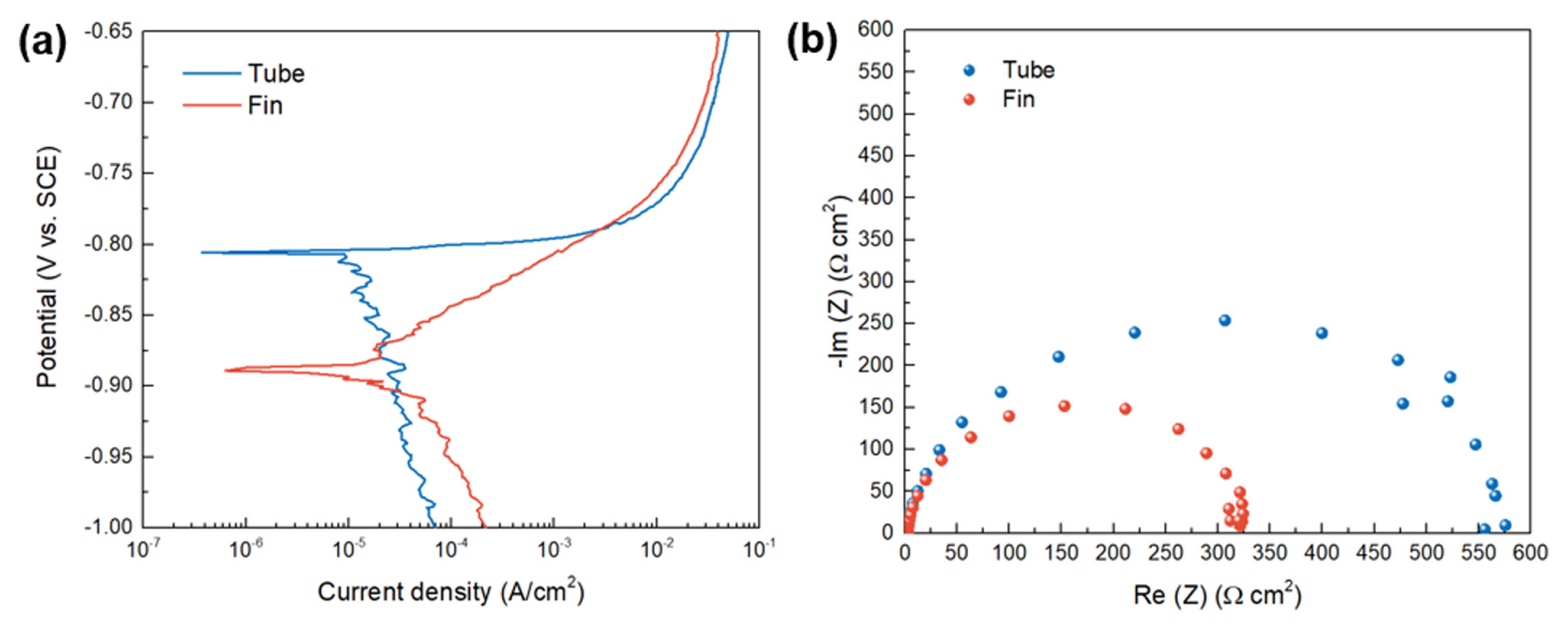
Fig. 4(a) illustrates the tube and fin polarization curves in a SWAAT solution. Specifically, the OCP of the tube was −0.806 V_SCE, whereas that of the fin was −0.885 V_SCE. Both materials showed active behaviors in the solution with corrosion current density of 10.6 μA/cm² for the tube, and 18.1 μA/cm² for the fin. EIS also showed the Randle circuit, R_s(Q_dlR_ct) [45]. This study modeled the capacitance using a constant phase element to obtain a better calculation between the model and experimental data. Thereafter, the impedance was defined using the following equation [46]:

(6)

ZCPE=Z0/(jw)n

where n ranges from −1 to 1, and Z₀ is a constant. For quantitative support and a better description of the experimental results, EIS parameters were obtained from ZSimpWin software and summarized in Table 3.

3.2.2 Filler metals

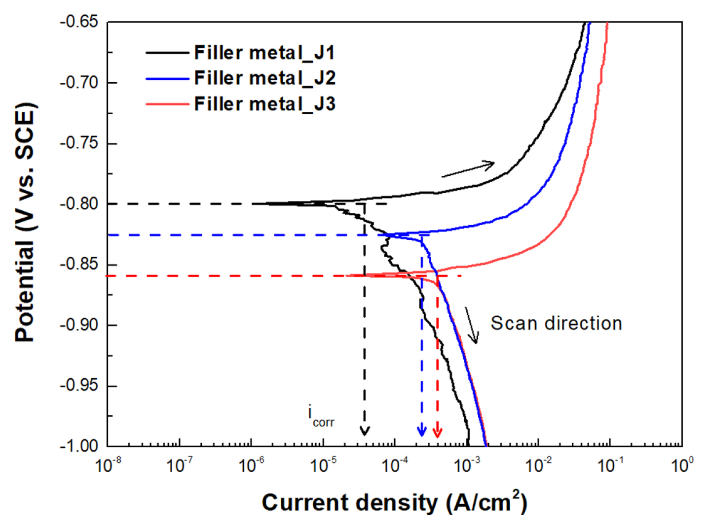
Fig. 5 presents the polarization curves of the filler metals in a SWAAT solution, from which the OCP, and corrosion current density of each alloy were determined. The OCP shifted to more negative values with an increase in Zn. Specifically, the OCP of J1 was −0.799 V_SCE, whereas those of J2, and J3 were −0.825 V_SCE and −0.860 V_SCE, respectively. This shift indicates the effect of Zn addition on the corrosion potential shift to negative values of the Al alloy. The corrosion current density increases as the corrosion potential decreases. Tafel extrapolation [21] was performed to evaluate the corrosion current density, which was found to be the lowest for J1 (37.7 μA/cm²), followed by J2 (238.0 μA/cm²) and J3 (384.0 μA/cm²), respectively. Si typically has a more noble potential than the Al matrix [47]; therefore, it can increase the corrosion current density of the alloy by acting as a local cathodic site [48]. However, as the Si content was controlled at the same level for each alloy, the influence of Si became insignificant compared to Zn addition. The enhanced reactivity of Al in chloride solutions containing Zn²⁺ can be attributed to several factors. These include the preferential dissolution of Zn [49], the increased instability of the Al oxide layer due to the formation of ZnAl₂O₄ [50], and the reduction in the pH of the oxide’s zero charge [51]. Consequently, introducing Zn elevates in the corrosion current density.

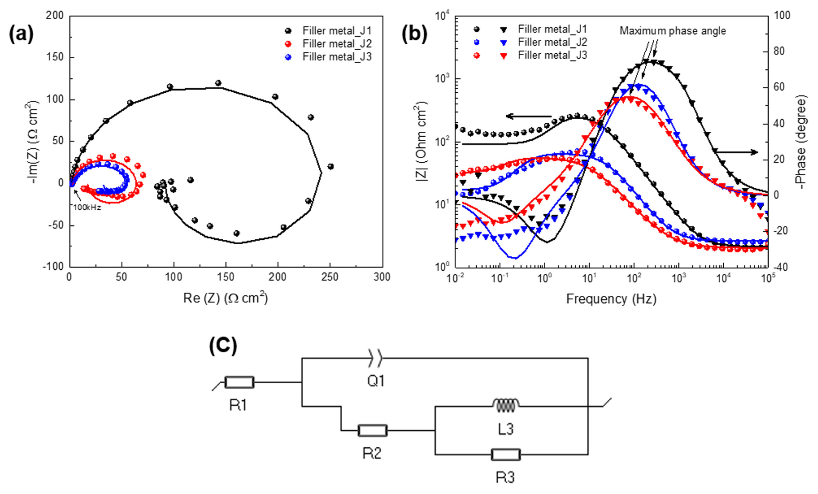
Fig. 6 displays the EIS test results as Nyquist and Bode plots. The Nyquist plots show one capacitive arc, which decreases in radius when Zn is added, and one inductive loop at relatively low frequencies, as shown in Fig. 6(a). The inductive loop at low frequencies can be attributed to the formation of intermediates when the alloy undergoes active dissolution. The inductive loops in the low-frequency region indicate that the reaction mechanism of dissolution involved elementary steps [52], associated with the adsorption of reaction intermediates during active dissolution [53]. The inductive loop can be measured due to the adsorption of species such as Zn(OH)₂ or Zn(OH)⁺ [24]. Furthermore, the decrease in the height of the maximum phase angle was associated with a reduction in the charge transfer resistance (R_ct), as shown in Fig. 6(b) [54]. The equivalent circuit model of the corrosion system in Fig. 6(c) was used to analyze the impedance plots accurately. This circuit consists of solution resistance (R₁), charge transfer resistance (R₂), double layer capacitance (Q₁), inductance (L₃), and resistance (R₃) of the adsorbed species. Table 4 shows that the polarization resistance (R_p), the sum of R₂, and R₃, differed significantly according to the Zn content. The R_p value was inversely proportional to the corrosion rate [21]. Therefore, the EIS analysis results showed that the corrosion rate of the alloy increased as the Zn content increased, as in the polarization test results. Moreover, due to the inductive loop, the impedance modulus from the Bode plots ranks as J1 > J3 > J2 at the lowest frequency, resulting in a different phase angle. At the lowest frequency, the impedance modulus (|Z|) represents the sum of R₁, R₂, R₃⁻¹ and (jwL₁)⁻¹. In this case, the difference R3 and L3 of J2 is larger than the J3, and the order of impedance modulus was changed compared with maximum phase angle (J1 > J2 > J3) at the lowest frequency.

3.3 Galvanic coupling of the Al heat exchanger

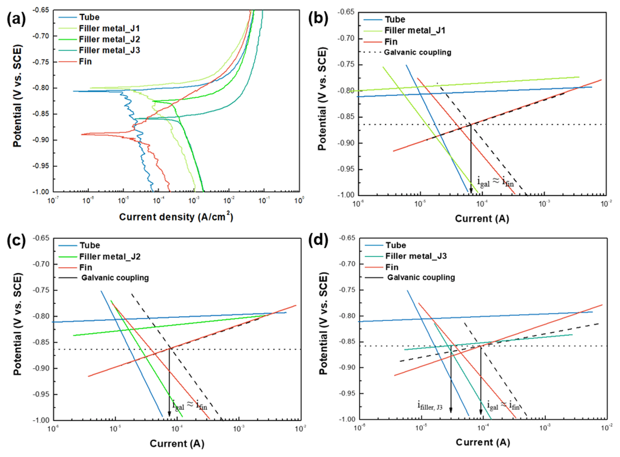
Fig. 7(a) presents the polarization curves of the fin, tube, and filler metals to evaluate the effect of galvanic corrosion of the heat exchanger, and the polarization parameters of each component alloy are listed in Table 5. The fin exhibited the most active corrosion potential with a value of −0.885 V_SCE, indicating that it can be used as the sacrificial anode. Conversely, the tube is designed to be the most protected component of the heat exchanger; thus, it has the most noble corrosion potential (−0.806 V_SCE) due to the risk of refrigerant leakage. Based on the corrosion potential of the tube, J2, and J3 alloys showed more active potential, while J1 exhibited more noble corrosion potential than the tube alloy. However, this study examined all three filler metal alloys to evaluate galvanic coupling in various designs. Fig. 7(b–d) show the results of the galvanic coupling considering the exposed area and the polarization data of each component. The data in Table 2 were used as a reference for the modeling results, and the polarization curves were extrapolated using the Tafel constant. The polarization curves were then added according to the mixed potential theory [55], and the total oxidation, and reduction current densities were used as the galvanic coupling curve, represented by the black dashed lines.

Fig. 7(b) presents the galvanic coupling of the tube–filler metal (J1)–fin (Case 1), where the corrosion potential order is J1 > tube > fin. The galvanic coupling potential, indicated by a dotted line, was −0.864 V_SCE. The oxidation and reduction reactions in each component were observed to equal the current values of the oxidation and reduction curves of each component at the intersection of the coupling potentials. Only the anodic curve of the fin alloy showed the intersection for the oxidation reaction, whereas for the reduction reaction, the cathodic curves of all three alloys intersected with the dotted line. Therefore, it was determined that the fin alloy acted as a sacrificial anode.

Fig. 7(c) shows the galvanic coupling of the tube–filler metal (J2)–fin (Case 2), where the potential order is tube > J2 > fin. The corrosion potential of J2 got closer to that of the fin as the Zn content of J2 increased. However, the corrosion current density of J2 also increased compared to that of J1. Therefore, the potential reduction effect between the fin and filler metal was not evident in Fig. 7(c). In this case, the galvanic coupling potential was −0.862 V_SCE, and a dotted line indicated the corresponding potential. Only the anodic curve of the fin alloy intersected the dotted line. For the reduction reaction, the cathodic curves of all three alloys intersected the dotted line. Therefore, the fin alloy functioned as a sacrificial anode, similar to the fin–J1–tube coupling.

In Contrast, Fig. 7(d) shows that the galvanic coupling of the tube–filler metal (J3)–fin (Case 3) exhibited different behavior in the anodic current density of the filler metal compared to the above two cases. In the tube–J3–fin coupling, an intersection occurred with a galvanic potential (−0.857 V_SCE) dotted line and the anodic curve of the J3 filler metal. In this case, the order of corrosion potential of the alloys matches the SACP design of tube > filler metal (J3) > fin. However, the corrosion potential of the J3 alloy was close to that of the fin alloy, and the corrosion current density of the J3 alloy was faster than that of the fin alloy. Therefore, even if the corrosion potential of the fin alloy was designed as a sacrificial anode, the filler metal alloy could experience an anodic reaction. Consequently, in the tri–metallic galvanic coupling, when the corrosion rate of the intermediate corrosion potential metal (filler metal) was faster than that of the sacrificial anode (fin), there was a risk of corrosion of the intermediate metal.

The galvanic potentials following the coupling cases were −0.864 V_SCE (Case 1), −0.862 V_SCE (Case 2), and −0.857 V_SCE (Case 3), respectively, lower than the corrosion potential of the tube. Therefore, the tube was cathodically protected in all cases. The reduced anodic current density of the tube was calculated based on the polarization parameters listed in Table 5. The anodic Tafel constant of the tube was 0.01 V/decade, indicating that when the potential of the tube was negatively polarized to 0.01 V, the anodic current density was reduced tenfold. Compared with the corrosion potential of the tube, the cathodic overpotentials with the galvanic coupling were −0.058 V (Case 1), −0.056 V (Case 2), and −0.051 V (Case 3), respectively. Therefore, the corrosion current densities of the tube (10.6 μA/cm²) were decreased by SACP to 0.017 nA/cm² (Case 1), 0.027 nA/cm² (Case 2), and 0.084 nA/cm² (Case 3), respectively. Consequently, the galvanic coupling reduced the corrosion current density by at least 10⁵ times, and Case 3 showed the most protective current density.

Compared with the corrosion potential of the fin, the anodic overpotentials with the galvanic coupling were 0.022 V (Case 1), 0.024 V (Case 2), and 0.029 V (Case 3), respectively. Therefore, the corrosion current densities of the fin (18.1 μA/cm²) were increased by SACP to 64.2 μA/cm² (Case 1), 72.0 μA/cm² (Case 2), and 96.1 μA/cm² (Case 3), respectively. Consequently, the fin acted as a sacrificial anode with galvanic coupling.

However, compared with the corrosion potential of the filler metals, the overpotentials with the galvanic coupling were −0.065 V (Case 1), −0.037 V (Case 2), and +0.003 V (Case 3), respectively. Therefore, the corrosion current densities of the filler metals were changed by galvanic coupling for SACP to 0.02 μA/cm² (Case 1), 14.0 μA/cm² (Case 2), and 483.4 μA/cm² (Case 3), respectively. Consequently, the corrosion current density of the filler metal (J3) increased with galvanic coupling.

3.4 Sacrificial anode cathodic protection simulation

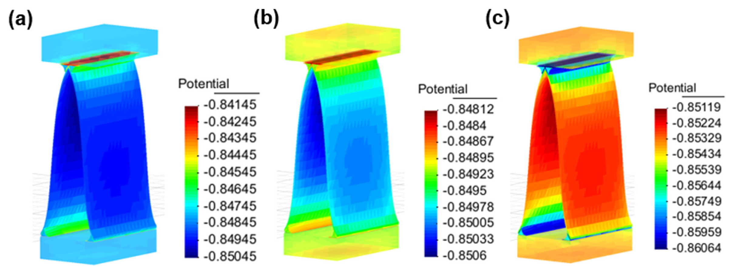
To predict and clarify the effect of geometrical factors on tri-metallic galvanic corrosion, computational simulation analyses were conducted using the BEASY software. The polarization parameters of each component alloy listed in Table 5 were used for the SACP simulation. The simulation results provide the distribution of potential and current density of the model. Fig. 8 presents the potential distribution results of each coupling case, and the maximum, and minimum galvanic potentials are summarized in Table 6. The tri-metallic galvanic coupling potential was lower than the corrosion potential of the tube in all cases. Additionally, no differences were observed in the distribution of the galvanic potential based on the distance in the tube modeling, as the conductivity of the electrolyte was sufficient, and the effect of SACP was well-operated. These results demonstrate that the tube was cathodically protected in all cases.

The galvanic potential decreases with more active filler metal. The maximum galvanic potentials for the filler metal models were −0.846 V_SCE (filler metal, J1), −0.848 V_SCE (filler metal, J2), and −0.857 V_SCE (filler metal, J3), respectively. Comparing the galvanic potential with the corrosion potential of each filler metal alloy (J1: −0.799 V_SCE, J2: −0.825 V_SCE, and J3: −0.860 V_SCE) showed that only the filler metal J3 represented the anodic polarization region. Moreover, when J1 and J2 alloys were used as filler metals, the corrosion potential of the tube showed a noble potential compared with its galvanic potential, and the corrosion potential of the fin only showed a more active potential than the galvanic potential, as shown in Fig. 8(a,b). Therefore, the fin will act as the sacrificial anode in these two cases. However, Fig. 8(c) shows that when J3 alloy was used as a filler metal, the corrosion potential of the filler metal and fin showed more active potential than the galvanic potential. Therefore, in this case, corrosion of the filler metal will occur.

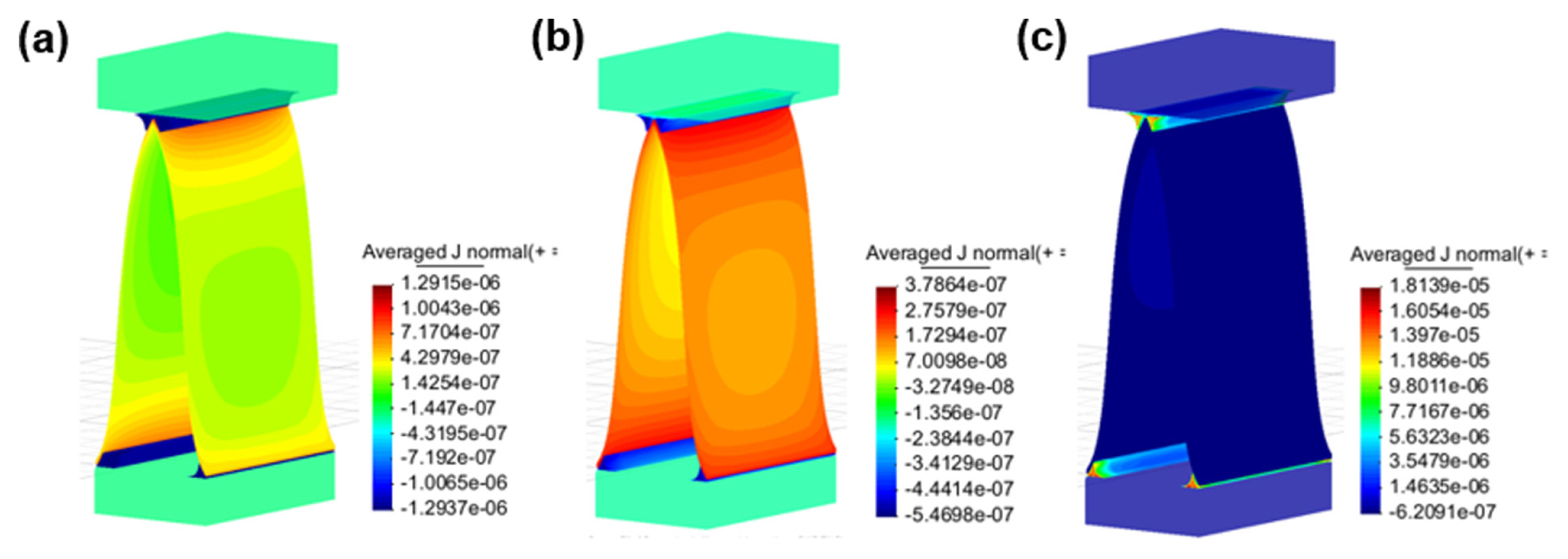
Additionally, the current density distribution was analyzed using the corrosion simulation, and the results are presented in Fig. 9. Similar to the potential distribution results, the tube and filler metal components showed negative current density, and the fin component displayed a positive current density. These results indicated that the fin alloy works effectively as a sacrificial anode when J1 and J2 alloys were used as filler metals. However, the simulation results showed a positive current density of the filler metal when the J3 alloy was used.

Table 6 lists the maximum and minimum values of the potential and current density for a detailed analysis of the corrosion simulation results. The potential difference between the components for each simulation case was insignificant. However, the simulation exhibited a significant difference in the current density. In Case 3, a significant active reaction of the filler metal and an overprotected tube component was observed. Meanwhile, the current density of the fin component in Cases 1 and 2 is noteworthy. The simulation of galvanic corrosion was conducted using the BEM–based mesh design and the electrochemical parameters of each material. In this case, the galvanic potentials, and currents at different locations in the simulation are influenced by the distance based on conductivity, which is derived from the electrochemical results of different materials. Consequently, even within a single component, different corrosion rates can be observed depending on the location. Although the heat exchanger represents a localized region influenced by separation or detachment, the factor that significantly affects its service life is the fastest corrosion rate value. Therefore, this study emphasized describing the maximum galvanic current density. In Case 1, the maximum current density of the fin was +129.0 μA/cm², whereas in Case 2, it was considerably smaller, at +37.8 μA/cm². These current densities were related to the lifespan of the heat exchanger product, with the current density of the fin indicating the consumption rate as the sacrificial anode of the fin. Therefore, considering the potential design of the heat exchanger and the lifetime of the sacrificial anode, it was most appropriate to use the J2 alloy as a filler metal.

4. Conclusions

To investigate the effect of Zn content in filler metal on SACP for suppressing tube corrosion, electrochemical tests, and computational corrosion simulation were performed for filler metals containing 0.5, 1.5, and 2.0 wt.% Zn. Increasing the Zn content of the filler metal decreased its corrosion potential toward the active region, which was expected to increase the lifespan of the heat exchanger by reducing the oxidation rate of the sacrificial anode (fin). However, the corrosion current density of filler metal also increased with an increase of Zn content. Notably, the corrosion current density of filler metal containing 2.0 wt.% Zn was significantly higher than that of the fin metal, resulting in filler metal corrosion despite the SACP design. Additionally, the oxidation rate of the fin with J1 (0.5 wt.% Zn) was faster than that with J2 (1.5 wt.% Zn) due to the significant potential difference between the fin and the filler metal. Therefore, the optimal Zn content for SACP was determined to be 1.5 wt.% in the filler metal, which maintained the cathodic protection of the tube and improved the lifespan of the heat exchanger in this alloy design.

The interpretation of galvanic coupling using the mixed-potential theory offers the advantage of considering both the corrosion potential and current density. However, it is limited to interpretating the galvanic potential drop solely based on locations. On the other hand, galvanic simulations are insufficient as they only consider the corrosion potential; however, they provide valuable insights into the variations in corrosion reactions of components based on distance, location, and conductivity. Therefore, considering both approaches were deemed effective in analyzing galvanic corrosion.

Acknowledgments

This research was supported by the Sungkyunkwan University and the BK21 FOUR (Graduate School Innovation) funded by the Ministry of Education (Korea) and National Research Foundation of Korea (NRF).

Notes

Author contributions

Yoon-Sik So: Conceptualization, Validation, Data curation, Writing-original draft, Writing-review & editing Eun-Ha Park: Formal analysis, Methodology, Resources Jung-Gu Kim: Writing-review & editing, Supervision

Fig. 1

Model for galvanic corrosion simulation: (a) image of the fin-tube Al heat exchanger; (b) magnified image of the white box in (a); (c) perspective image; (d) front image.

Fig. 2

Boundary conditions for the galvanic corrosion simulation of the fin-tube Al heat exchanger.

Fig. 3

Microstructure and precipitate analyses of the filler metals using scanning electron microscopy: (a) 0.5 wt.% Zn, (b) 1.5 wt.% Zn, (c) 2.0 wt.% Zn, (d) EDS result of the light gray particle, and (e) EDS result of the bright particle in (c).

Fig. 4

(a) Polarization curves, and (b) Nyquist plots of the tube and fin in the sea water acetic acid test (SWAAT) solution at 49°C.

Fig. 5

Polarization curves of the filler metals as a function of zinc content in the sea water acetic acid test (SWAAT) solution at 49°C.

Fig. 6

Experimental impedance spectra of the filler metals in the seawater acetic acid test solution, (a) Nyquist plots, (b) Bode plots, and (c) equivalent circuit.

Fig. 7

Tafel plots of the polarization curves with the calculated area of the fin–tube Al heat exchanger coupling alloys in the seawater acetic acid test solution, (a) polarization curves of the tube, filler metals, and fin alloy, (b) tube–filler metal (J1)–fin (Case 1), (c) tube–filler metal (J2)–fin (Case 2), and (d) tube–filler metal (J3)–fin (Case 3) coupling.

Fig. 8

Galvanic potential distribution of each simulation case: (a) tube–filler metal (J1)–fin (Case 1), (b) tube–filler metal (J2)–fin (Case 2), and (c) tube–filler metal (J3)–fin (Case 3).

Fig. 9

Galvanic current distribution of each simulation: (a) tube–filler metal (J1)–fin (Case 1), (b) tube–filler metal (J2)–fin (Case 2), and (c) tube–filler metal (J3)–fin (Case 3).

Table 1

Chemical compositions of Al alloys for heat exchanger

		Chemical composition (wt.%)

Alloy		Mn	Fe	Si	Cu	Zn	Zr	Al

Tube		0.5	≤0.1	-	-	-	0.15	Bal.

Filler metal	J 1	-	≤0.1	7.5	≤0.1	0.5	-
	J 2					1.5
	J 3					2.0

Fin		1.2	0.7	0.6	0.3	2.5	-

Table 2

Conditions of the scale of the model

Part	Width (mm)	Length (mm)	Height (mm)	Shape	Total surface area (mm²)
Tube	3.0	5.0	1.0	Rectangular	92
Filler metal	0.3	5.0	0.3	Triangular prism	6.36
Fin	0.1	5.0	8.0	Thin sheet	166

Table 3

Results of the EIS test of the tube and fin

	R_s	Q_dl		R_ct	R_p

	Ωcm²	μF/cm²	n	Ωcm²	Ωcm²
Tube	1.20	41.64	0.93	605.0	603.7
Fin	2.59	25.26	0.96	324.9	322.3

Table 4

Results of the EIS test of the filler metals

	R₁	Q₁		R₂	L₃	R₃	R_p

	Ωcm²	μF/cm²	N	Ωcm²	Hcm²	Ωcm²	Ωcm²
J1	2.15	44.50	0.94	89.81	12.08	165.8	255.61
J2	2.66	148.20	0.94	34.70	18.76	27.58	62.28
J3	2.05	538.60	0.83	30.38	24.90	24.89	55.27

Table 5

Polarization parameters of each component alloy used for the corrosion simulation

Alloy		Corrosion potential (V_SCE)	Corrosion current density (μA/cm²)	Anodic Tafel slope (V/Decade)	Cathodic Tafel slope (V/Decade)

Tube		−0.806±0.005	10.6±0.8	0.01	0.24±0.01

Filler metal	J1	−0.799±0.012	37.7±3.6	0.02	0.23±0.01
	J2	−0.825±0.009	238.0±12.5	0.03	0.24±0.01
	J3	−0.860±0.013	384.0±10.8	0.03	0.27±0.01

Fin		−0.885±0.007	18.1±1.1	0.04	0.26±0.01

Table 6

Maximum and minimum values of the galvanic potential and current density evaluated using the corrosion simulation

Simulation case	Part	Galvanic potential (V_SCE)		Galvanic current density (μA/cm²)		Polarization state from simulation

		Max.	Min.	Max.	Min.
1	Tube	−0.847	−0.847	−14.5	−14.5	Cathode
	J1	−0.846	−0.846	−129.0	−129.0	Cathode
	Fin	−0.850	−0.850	+129.0	+14.2	Anode

2	Tube	−0.848	−0.849	−13.6	−13.6	Cathode
	J2	−0.848	−0.849	−34.1	−54.6	Cathode
	Fin	−0.847	−0.850	+37.8	+7.0	Anode

3	Tube	−0.853	−0.854	−146.0	−146.0	Cathode
	J3	−0.857	−0.860	+1810.0	+354.0	Anode
	Fin	−0.851	−0.854	+146.0	+62.1	Anode

References

[1] A. C. caket, C. Wang, M. A. Nugroho, H. Celik and M. Mobedi, Renew. Sust. Energy Rev., 2022, 167, https://doi.org/10.1016/j.rser.2022.112697 .

[2] M. G. Schmidt, H. H. Attaway, S. Terzieva, A. Marshall, L. L. Steed, D. Salzberg, H. A. Hamoodi, J. A. Khan, C. E. Feigley and H. J. Michels, Curr. Microbiol., 2012, 65(2), 141–149.

[3] D. Junqi, Z. Yi, L. Gengtian and X. Weiwu, Exp. Heat Tranf., 2013, 26(4), 384–396.

[4] A. Burlacu, G. Sosoi, R. S. Vizitiu, M. Bărbută, C. D. Lăzărescu, V. Ciocan and A. Serbănoiu, Procedia Manuf., 2018, 22, 714–721.

[5] H. Fugmann, E. Laurenz and L. Schnabel, Energies, 2017, 10(9), 1341.

[6] A. Nuntaphan, S. Vithayasai, N. Vorayos, N. Vorayos and T. Kiatsiriroat, Int. Commun. Heat Mass Transf., 2010, 37(3), 287–292.

[7] K. M. Shirvan, R. Ellahi, S. Mirzakhanlari and M. Mamourian, Appl. Therm. Eng., 2016, 109, 761–774.

[8] J. Zhang, X. Zhu, M. E. Mondejar and F. Haglind, Renew. Sustain. Energy Rev., 2019, 101, 305–328.

[9] X. Guo, Y. Fan and L. Luo, Energy, 2014, 69, 728–741.

[10] F.-J. Chen, C. Yao and Z.-G. Yang, Eng. Fail. Anal., 2014, 37, 42–52.

[11] M. S. Hong, I. J. Park and J. G. Kim, Met. Mater. Int., 2017, 23, 708–714.

[12] B. Badenes, B. Sanner, M. Á. M. Pla, J. M. Cuevas, F. Bartoli, F. Ciardelli, R. M. González, A. N. Ghafar, P. Fontana, L. L. Zuniga and J. F. Urchueguía, Energy, 2020, 201, 117628.

[13] K. Iijima, T. Miura, Y. Hasegawa, Y. Baba, Z. Tanabe and M. Hagiwara, SAE Transaction 1986, 95, 482. –488 https://www.jstor.org/stable/44721674 .

[14] M. Pech-Canul, J. C. Guía-Tello, M. I. Pech-Canul, J. C. Aguilar, J. A. Gorocica-Díaz, R. Arana-Guillén and J. Puch-Bleis, Results Phys., 2017, 7, 1760–1777.

[15] S.-J. Ko, J.-H. An, Y.-S. Kim and J.-G. Kim, Eng. Fail. Anal., 2019, 98, 167–176.

[16] L. Shi, Y. Song, P. Zhao, H. Wang, K. Dong, D. Shan and E.-H. Han, Electrochim. Acta, 2020, 359, 136947.

[17] R. Akid and D. J. Mills, Corros. Sci., 2001, 43(7), 1203–1216.

[18] L. Shi, Y. Song, K. Dong, H. Wang, D. Shan and E.-H. Han, Corros. Sci., 2021, 184, 109400.

[19] C. Vargel, Corrosion of Aluminium. Elsevier, 2020. p.149–153.

[20] Z.-Z. Yan, Q.-H. Zhang, H.-R. Cai, X.-R. Li, L.-K. Wu, Z.-Z. Luo and F.-H. Cao, Corros. Sci., 2022, 206, 110541.

[21] Y.-S. Kim, I.-J. Park and J.-G. Kim, Metals, 2019, 9(3), 376.

[22] Y. Tang, L. Lu, H. W. Roesky, L. Wang and B. Huang, J. Power Sources, 2004, 138(1–2), 313–318.

[23] S. Khireche, D. Boughrara, A. Kadri, L. Hamadou and N. Benbrahim, Corros. Sci., 2014, 87, 504–516.

[24] M. A. Amin, S. S. Abd El-Rehim, E. E. F. El-Sherbini, S. R. Mahmoud and M. N. Abbas, Electrochim. Acta, 2009, 54(18), 4288–4296.

[25] Q. F. Hu, T. Zhang, S. J. Geng and F. H. Wang, Mater. Corros., 2017, 68(9), 935–942.

[26] J. Liu, X. Huang, Y. Ren, L. M. Wong, H. Liu and S. Wang, Sci. Rep., 2022, 12, 4532.

[27] K. Thekkepat, H.-S. Han, J.-W. Choi, S.-C. Lee, E. S. Yoon, G. Li, H.-K. Seok, Y.-C. Kim, J.-H. Kim and P.-R. Cha, J. Magnes. Alloys, 2022, 10(7), 1972–1980.

[28] T. Kosaba, I. Muto and Y. Sugawara, J. Electrochem. Soc., 2022, 169, 020550.

[29] J. Hazarika, A. Gupta and P. V. Rajaraman, ECS J. Solid State Sci. Technol., 2022, 11, 054007.

[30] K. Kondoh, R. Takei, S. Kariya, S. Li and J. Umeda, Mater. Lett., 2022, 319, 132266.

[31] D. A. Jones, Principles and Prevention of Corrosion. 2nd ed. Prentice-Hall, USA, 1992. p.86–92.

[32] G. Song, B. Johannesson, S. Hapugoda and D. StJohn, Corros. Sci., 2004, 46(4), 955–977.

[33] M.-C. Zhao, M. Liu, G. L. Song and A. Atrens, Adv. Eng. Mater., 2008, 10(1–2), 104–111.

[34] Y.-S. So, J.-M. Lim, N. T. Chung and J.-G. Kim, Corrosion, 2023, 79(7), 790–801.

[35] F. N. Afshar, J. H. W. de Wit, H. Terryn and J. M. C. Mol, Corros. Sci., 2012, 58, 242–250.

[36] Y.-S. Kim, J. G. Park, B.-S. An, Y. H. Lee, C.-W. Yang and J.-G. Kim, Materials, 2018, 11(10), 1982.

[37] R. A. Adey and S. M. Niku, Computer modelling of galvanic corrosion. In: H. P Hack editors. Galvanic corrosion, ASTM STP 978. American Society for Testing and Materials, PA, USA, 1988. p.96–117.

[38] P. Biswas, S. Patra and M. K. Mondal, Int. J. Cast Met. Res., 2020, 33(2–3), 134–145.

[39] Q. Miao, D. Wu, D. Chai, Y. Zhan, G. Bi, F. Niu and G. Ma, Mater. Des., 2020, 186, 108205.

[40] A. G. Muñoz, S. B. Saidman and J. B. Bessone, Corros. Sci., 2002, 44(10), 2171–2182.

[41] M. Nestoridi, D. Pletcher, R. J. K. Wood, S. Wang, R. L. Jones, K. R. Stokes and I. Wilcock, J. Power Sources, 2008, 178(1), 445–455.

[42] M. Qian, D. Li, S. B. Liu and S. L. Gong, Corros. Sci., 2010, 52(10), 3554–3560.

[43] D. Jiang and J. Yu, J. Mater. Res. Technol., 2019, 8(3), 2930–2943.

[44] S.-I. Pyun and W.-J. Lee, Corros. Sci., 2001, 43(2), 353–363.

[45] W. Choi, H.-C. Shin, J. M. Kim, J.-Y. Choi and W.-S. Yoon, J. Electrochem. Sci. Technol., 2020, 11(1), 1–13.

[46] Y.-P. Xiao, Q.-L. Pan, W.-B. Li, X.-Y. Liu and Y.-B. He, Mater. Des., 2011, 32(4), 2149–2156.

[47] K. Mizuno, A. Nylund and I. Olefjord, Corros. Sci., 2001, 43(2), 381–396.

[48] V. Guillaumin and G. Mankowski, Corros. Sci., 2000, 42(1), 105–125.

[49] S. B. Saidman, A. G. Munoz and J. B. Bessone, J. Appl. Electrochem., 1999, 29, 245–251.

[50] C. B. Breslin and L. P. Friery, Corros. Sci., 1994, 36(2), 231–240.

[51] P. M. Natishan, E. McCafferty and G. K. Hubler, J. Electrochem. Soc., 1988, 135, 321.

[52] M. Itagaki, A. Taya, K. Watanabe and K. Noda, Anal. Sci., 2002, 18, 641–644.

[53] S. M. A. Shibli and S. George, Appl. Surf. Sci., 2007, 253(18), 7510–7515.

[54] Y. Deng, Z. Yin, K. Zhao, J. Duan, J. Hu and Z. He, Corros. Sci., 2012, 65, 288–298.

[55] G. S. Frankel, Fundamentals of corrosion kinetics. In: A Hughes, J Mol, M Zheludkevich, R Buchheit editors. Active protective coatings. Springer, Netherlands, 2016. p.17–32.